We have built a strong material to reach this stage, the five post series on uncertainty is the building block for understanding probabilistic approach to deep learning and the efficacy of log-likelihood ratio as a loss function. Further, we assessed the importance of Jacobian matrix in optimization convergence, refer…

• Uncertainty - A series of 5 articles covers the fundamentals
• Calculus - Gradient Descent Optimization through Jacobian Matrix for a Gaussian Distribution

Image Credit: Probabilistic Deep Learning with TensorFlow 2

Before any theory, we'll discuss an example of how normalizing flows work. Suppose you have a standard normal 
distribution (mean 0, variance 1). It has a single mode at 0, so, even after scaling and shifting, can't be 
fit well to data with two modes. However, the bijectors applied to distributions can create other distributions. 
A natural question is then: can we create a bimodal distribution (one with two modes) from a bijector applied 
to a standard normal distribution? It turns out that this is possible with the `Softsign` bijector. This is a 
differentiable approximation to the sign function (1 if x is nonnegative, -1 if x is negative). Passing a 
standard normal distribution through this bijector transforms the probability distribution as above
- Kevin Webster et al, Imperial College London

Objective

The key objective of this post is to build a foundation for density estimation using normalizing flows by

• Understand the concept of normalizing flows
• Explore the math and intuition behind normalizing flows
• Significance of Determinant of the Jacobians
• Construct a flow architecture using Bijectors
• Chain the bijectors and make transformations
• Visualize the transformation at each step from base distribution to the most sophisticated one.

Introduction

It is not normal to be normal in the real world, reality is a dynamic, reflexive, non-linear chaotic system. There is absolutely nothing fits under the normal distribution. However, we using Gaussian distribution as the starting point for most of the real world problems because the embedded probability distribution is simple enough to calculate the derivatives easily in the backpropagation stage of DNN. To address this shortcoming and to achieve more powerful distribution approximations, Normalizing Flow models are recommended.

A Normalizing Flow is a transformation of a simple probability distribution(e.g. a standard normal) into a 
more complex distribution by a sequence of invertible and differentiable mappings.
The density of a sample can be evaluated by transforming it back to the original simple distribution.
- Kobyzev et al, Normalizing Flows: An Intro and Review of Current Methods

This mechanism makes it easy to construct new families of distributions by choosing initial densities and then chaining with parameterized, invertible and differentiable transformations.

$$\Large z_0 \sim p_0(z_0) \tag{1. Base Distribution}$$

Where, $p_0$ is the density of the base distribution.

Normalizing Flows should satisfy several conditions in order to be practical. They should:

• be invertible; for sampling we need function and for computing likelihood we need another function,
• be sufficiently expressive to model the distribution of interest,
• be computationally efficient, both in terms of computing f and g (depending on the application) but also in terms of the calculation of the determinant of the Jacobian.

Image Credit: Flow-based Deep Generative Models

Based on the figure which is an absolute representation of Kobyzev et al, $$z_{i-1} \sim p_{i-1}(z_{i-1}) \tag{2}$$

$$z_i = f_i(z_{i-1})$$ $$thus$$ $$z_{i-1} = f_i^{-1}(z_i)$$ $$from \ eqn.2$$ $$p_i(z_i) = p_{i-1}(f_i^{-1}(z_i))\left| det \frac{df_i^{-1}}{dz_i} \right| \tag{3}$$

In $eqn.3$ the basic rule for transformation of densities considers an invertible, smooth mapping $f: \mathcal{R}^d \rightarrow \mathcal{R}^d$ with inverse $f^{-1}$. This mapping is used to transform the random variable(simple distribution) to obtain a new density.

Applying the chain rule of inverse function theorem which is a property of Jacobians of invertible functions, we can construct arbitrarily complex densities by composing several simple maps of successive application.

$$p_i(z_i) = p_{i-1}(z_{i-1})\left| det \left(\frac{df_i}{dz_{i-1}}\right)^{-1} \right|$$

We are dealing with very small numbers, hence we shall move to log spaces $$log p_i(z_i) = log p_{i-1}(z_{i-1}) + log \left| det \left(\frac{df_i}{dz_{i-1}}\right)^{-1} \right|$$

$$log p_i(z_i) = log p_{i-1}(z_{i-1}) - log \left| det \frac{df_i}{dz_{i-1}} \right| \tag{4}$$

the final term is the ‘determinant of the Jacobian’

Elementwise Flow: Intuition

We shall generalize the $eqn.4$, A normalizing flow consists of invertible mappings from a simple latent distribution $p_z(z)$ to a complex distribution $p_x(x)$. As we have seen before, $f_i$ be an invertible transformation from $z_{i-1} to z_i, z_0 = z$. Then the log-likelihood $log p_X(x)$ can be expressed in terms of the latent variable z based on the change of variables theorem.

$$z = f_1^{-1} \circ f_2^{-1} \circ \cdots f_k^{-1}(x) \tag{5}$$ $$from \ eqn.4$$ $$logp_X(x) = log p_Z(z) - \sum_{i=1}^k log \left| det \left( \frac{\partial f_i}{\partial z_{i-1}} \right) \right| \tag{6. Log Likelihood}$$

$eqn. 5, 6$ suggests that that optimization of flow-based models requires the tractability of computing $f^{-1}$ and $log \left| det \left( \frac{\partial f_i}{\partial z_{i-1}} \right) \right|$. After training, sampling process can be performed efficiently as follows

$$z \sim p_Z(z)$$ $$x = f_k \circ f_{k-1} \circ \cdots f_1(z) \tag{8}$$

Flow Architecture

The normalizing flow demonstrated in this article has 5 transformations along with the base distribution as 2D Gaussian function. Using this function, we shall sample images in the subsequent sections.

• Base Distribution with a random variable of specified mean$(\mu)$ and standard deviation$(\sigma)$
  and the transformations as follows
• $f_1(z) = (z_a + c_0, z_b + c_1)$ and $c \in \mathbb{R}$
• $f_2(z) = (z_a \times d_0, z_b \times d_1)$ and $d \in \mathbb{R}$
• $f_3(z) = (z_a, z_b + ez_1^3)$ and $e \sim N(i, j)$ where $i, j \in \mathbb{R}$
• $f_4(z) = \mathbb{R}z$, where $\mathbb{R}$ is a rotation matrix with angle $\theta$
• $f_5(z) = sigmoid(z)$, sigmoid function is applied elementwise

Then the transformed random variable x is $$x = f_5 \circ f_4 \circ f_3 \circ f_2 \circ f_1(z) \tag{9}$$

Constructing the Flow

In this section, we shall construct the flow using bijectors and other functions of tensorflow probability library

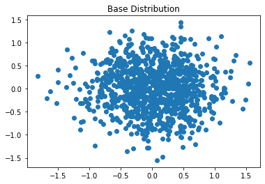
Base Distribution

In this section, let us build a base distribution and sequence of invertible tranformation functions to arrive at a powerful distribution approximation using Bijectors of Tensorflow Probability(TFP) library.

Let us say a 2D Gaussian random variable $z_0=(z_a, z_b)$ with $\mu=0, \sigma=0.5$ and the base distribution constructed as follows…

import numpy as np
import tensorflow as tf
import tensorflow_probability as tfp
tfd = tfp.distributions
def create_2d_gaussian(𝜇=0, 𝜎=0.5):
    return tfd.MultivariateNormalDiag(
        loc=[𝜇, 𝜇],
        scale_diag=[𝜎, 𝜎]
    )

import matplotlib.pyplot as plt
%matplotlib inline

gaussian_2d_base_dist = create_2d_gaussian()
gaussian_2d_samples = gaussian_2d_base_dist.sample(1000)
plt.scatter(gaussian_2d_samples[:, 0], gaussian_2d_samples[:, 1])
plt.title("Base Distribution")
plt.show()

Shift $f_1(z) = (z_a + c_0, z_b + c_1)$

Transformation one has shift functionality, build a utility function to perform the same.

This image is to understand the shift logic, not implemented as per the visual
Image Credit: Using Transformations to Graph Functions

def f1(c1=0, c2=-2):
    return tfb.Shift([c1, c2])

Scale $f_2(z) = (z_a \times d_0, z_b \times d_1)$

Scale at the provided dimensions

Image Credit: Scale

def f2(d1=1, d2=0.5):
    return tfb.Scale([d1, d2])

Shift and Cube $f_3(z) = (z_a, z_b + ez_1^3)$

Shift and Cube the distribution

tfb = tfp.bijectors
class ShiftAndCube(tfb.Bijector):
    def __init__(self, validate_args=False, name="Shift and Cube"):
        super(ShiftAndCube, self).__init__(
            validate_args=validate_args,
            forward_min_event_ndims=1,
            inverse_min_event_ndims=1,
            name=name,
            is_constant_jacobian=True
        )
        self.a = tfd.Normal(loc=3, scale=1).sample()

    def _forward(self, x):
        x = tf.cast(x, tf.float32)
        a = [
             [0, self.a],
             [0, 0]
        ]
        return x + tf.matmul(tf.pow(x, 3), a)


    def _inverse(self, y):
        y = tf.cast(y, tf.float32)
        a = [
             [0, self.a],
             [0, 0]
        ]
        return y - tf.matmul(tf.pow(y, 3), a)

    def _forward_log_det_jacobian(self, x):
        return tf.constant(1, dtype=tf.float32)
    
def f3():
    return ShiftAndCube()

Rotate $f_4(z) = \mathbb{R}z$

Rotate the distribution by an angle $\theta$

class Rotation2D(tfb.Bijector):
    def __init__(self, validate_args=False, name="rotation_2d"):
        super(Rotation2D, self).__init__(
            validate_args=validate_args,
            forward_min_event_ndims=1,
            inverse_min_event_ndims=1,
            name=name,
            is_constant_jacobian=True
        )

        theta = tfd.Uniform(low=0.0, high=2*np.pi).sample()

        self.cos_theta = tf.math.cos(theta)
        self.sin_theta = tf.math.sin(theta)
        self.event_ndim = 1

    def _forward(self, x):
        batch_ndim = len(x.shape) - self.event_ndim
        x0 = tf.expand_dims(x[..., 0], batch_ndim)
        x1 = tf.expand_dims(x[..., 1], batch_ndim)
        y0 = self.cos_theta * x0 - self.sin_theta * x1
        y1 = self.sin_theta * x0 - self.cos_theta * x1

        return tf.concat((y0, y1), axis=-1)

    def _inverse(self, y):
        batch_ndim = len(y.shape) - self.event_ndim
        y0 = tf.expand_dims(y[..., 0], batch_ndim)
        y1 = tf.expand_dims(y[..., 1], batch_ndim)
        x0 = self.cos_theta * y0 + self.sin_theta * y1
        x1 = -self.sin_theta * y0 + self.cos_theta * y1
        return tf.concat((x0, x1), axis=-1)

    def _forward_log_det_jacobian(self, x):
        return tf.constant(0., x.dtype)
    
def f4():
    return Rotation2D()

Sigmoid $f_5(z) = Sigmoid(z)$

def f5():
    return tfb.Sigmoid()

bijectors = [f1(), f2(2, 1.5), f3(), f4(), f5()]
names = [
    f'$f(z) = (z_a, z_b + c) \\rightarrow Shift$', 
    f'$f(z) = (z_a, z_b x d) \\rightarrow Scale$',
    f'$f(z) = (z_a, z_b + ez_1^3) \\rightarrow Shift & Cube$',
    f'$f(z) = Rz \\rightarrow Rotate$',
    f'$f(z) = Sigmoid(z)$'
]

def create_transformed_distribution(base_distribution, bij):
    bijector = tfb.Chain(list(reversed(bij)))
    
    transformed_distribution = tfd.TransformedDistribution(
        distribution=base_distribution,
        bijector=bijector
    )
    return transformed_distribution

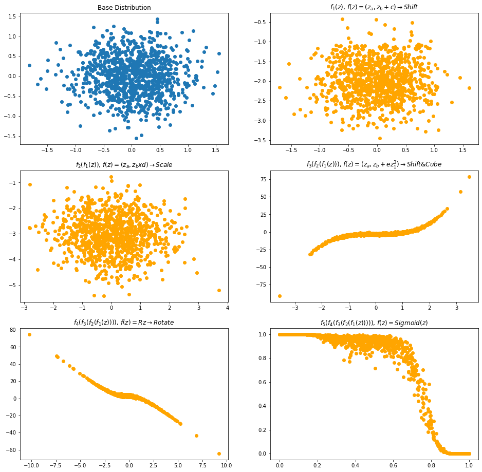
Visualize the Density Transformation

Using the random normalizing flow, we are generating the image dataset. Let us plot the change in density at as we apply transformation of the 5 functions of our architecture. i.e. Visualization at every stage of the equation $$x = f_5 \circ f_4 \circ f_3 \circ f_2 \circ f_1(z)$$

def plot_flow_densities(base_sample, base_dist, bijectors, names):
    _, axs = plt.subplots(3, 2, figsize=(16, 16))
    row = 0
    col = 0
    axs[row, col].scatter(base_sample[:, 0], base_sample[:, 1])
    axs[row, col].set_title("Base Distribution")
    col = 1
    function = 'z'
    func = 1
    for i in np.arange(1, 6):
        transformed_dist = create_transformed_distribution(base_dist, bijectors[0:i])
        img = transformed_dist.sample(1000)
        ax = axs[row, col]
        ax.scatter(img[:,0], img[:,1], color="orange")
        
       
        function = f'f_{func}({function})'
        ax.set_title(f'${function}$, {names[i-1]}')
        func += 1
        if(i % 2 == 1):
            row += 1
            col = 0
        else:
            col = 1
    plt.show()
    
plot_flow_densities(gaussian_2d_samples, gaussian_2d_base_dist, bijectors, names)

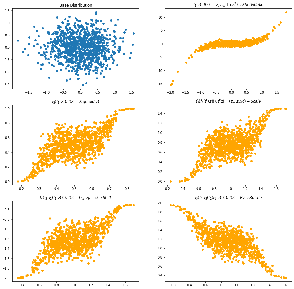
from sklearn.utils import shuffle
X, y = shuffle(bijectors, names)
plot_flow_densities(gaussian_2d_samples, gaussian_2d_base_dist, X, y)

X, y = shuffle(bijectors, names)
plot_flow_densities(gaussian_2d_samples, gaussian_2d_base_dist, X, y)

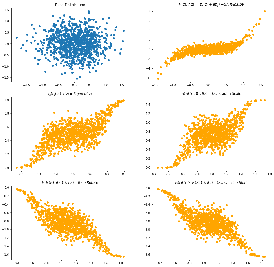
Inference

In this post, we did end-to-end coding for achieving a sample normalizing flow architecture. This is the first step towards understanding and building density estimation models for generative problems. As part of this, we transformed the base distribution to a sophisticated distribution using bijectors. In the visualization section, we shuffled the bijectors and created new distributions from the same set of functions. This post will pave way for us to explore some of the exciting concepts like

• Density estimation using RealNVP, real valued non-volume preserving transformations
• NICE: Non-Linear Independent Components Estimation
• MADE: Masked Autoencoder for Distribution Estimation

Reference

• Normalizing Flows Tutorial, Part 1: Distributions and Determinants
  by Eric Jank, 2018
• Normalizing Flows: An Introduction and Review of Current Methods
  Kobyzev et all, IEEE Transaction on Pattern and Machine Intelligence, 2020
• SoftFlow: Probabilistic Framework for Normalizing Flow on Manifolds
  Kim et all, NeurIPS, 2020
• Flow-based Deep Generative Models
  by Lilian Weng, 2018
• Normalizing Flows
  by Lukas Rinder
• Gaussianization Flows
  Meng et al, Stanford University, 2020
• Awesome Normalizing Flows
  by Janosh Riebesell
• MADE: Masked Autoencoder for Distribution Estimation Germain et al, Deep Mind etc, 2015
• Normalizing Flows - Motivations, The Big Idea, & Essential Foundations
  by Kapil Sachdeva, 2021
• Normalizing Flows
  by Adam Kosiorek, 2018
• Variational Inference with Normalizing Flows
  by Rezende et at, Deep Mind, 2016