This is a foundational topic that naturally leads to statistical representation of data using means and variances, geometrical representation of vector spaces, projection of data into lower dimensional sub-space and dimensionality reduction. However, we are quite focusing on the various properties of a covariance matrix and it’s significance on optimization.

I thank Prof. Jim Fowler of The Ohio State University, Without his Calculus 1/2/3 courses these posts would’nt have seen the light

Image Credit: Demystifying Optimizations for machine learning

This post is part of Math for AI/ML series, other previous posts are

• Roll your sleeves! Let us do some partial derivatives.
• Automatic Differentiation Using Gradient Tapes
• Calculus - Gradient Descent Optimization through Jacobian Matrix for a Gaussian Distribution

Objective

We want to understand 2 key properties of a covariance matrix.

• Positive Definite
• Positive Semi-Definite
• What is the significance of these 2 terms

Introduction

Covariances indicates the relationship between feature vectors, a positive covariance means the features moves together and a negative covariance indicates inverse move. This section has 4 parts

• Geometric intepretation of a covariance matrix
• Positive Definite - Mathematical Interpretation
• Positive Semi-Definite - Mathematrical Interpretation
• Properties of a Covariance Matrix

Geometric Interpretation of a Covariance Matrix

Why this property positive semi-definite is critical in machine learning… Here you go with a geometric interpretation

• If a matrix is positive definite, It has an absolute minima minima. What I meant by absolute minima, we achieved minima at all axis.
• If a matrix is positive semi-definite, It has a minima in at least one axis vector
• If a matrix is negative definite, It is an absolute maxima
• If a matrix is negative semi-definite, It has a maxima in at least one axis vector
• If a matrix is indfinite, It is a saddle point

import matplotlib.image as mpimg
fig, ax = plt.subplots(3, 2, figsize=(12, 12))
ax[0, 0].imshow(mpimg.imread("positive_definite.png"))
ax[0, 0].set_title("Positive Definite: Absolute Minima", fontsize=16)
ax[0, 1].imshow(mpimg.imread("positive_semi_definite.png"))
ax[0, 1].set_title("Positive Semi-Definite: Minima on an Axis", fontsize=16)
ax[1, 0].imshow(mpimg.imread("negative_definite.png"))
ax[1, 0].set_title("Negative Definite: Absolute Maxima", fontsize=16)
ax[1, 1].imshow(mpimg.imread("negative_semi_definite.png"))
ax[1, 1].set_title("Negative Semi-Definite: Maxima on an Axis", fontsize=16)
ax[2, 0].imshow(mpimg.imread("indefinite.png"))
ax[2, 0].set_title("Indefinite: Saddle Point", fontsize=16)
plt.show()

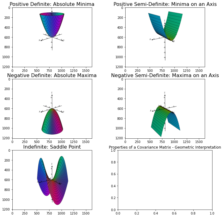
Image Credit: Ximera, OSU - Categorizing Quadratic Forms

Those images say n number of stories, when we have multiple feature vectors… a global minima can be obtained through intersections of multiple positive semi-definite matrices of different feature vectors. Refer this post for better clarity on minimas and maximas,

• Calculus - Gradient Descent Optimization through Jacobian Matrix for a Gaussian Distribution

This blog post is full of definitions and proofs on foundational concepts of vector representation of data, i.e. matrix.

• Symmetric Matrix: if $A = A^T$ i.e. A matrix is symmetric if it is equal to its transpose
• Matrix Congruence: Two square matrices $(A, B)$ are congruent if there exists an invertible matrix P then $P^TAP = B$

Positive Definite

We have 3 definitions for positive-definite

• Through the nature of the input vector
• Through it’s eigen vectors
• Through a rectangular matrix R with independent columns

Definition 1
A $n \times n$ symmetric matrix $M$ is positive-definite, if $$x^TMx \gt 0 \tag{1. +ve Definite}$$ for all non-zero $x \in \mathbb{R}^{1 \times n}$, that is a $1 \times n$ column vector.

Through Eigen Values
A matrix is positive definite if it’s symmetric and all its eigenvalues are poitive.
We shall see this in the future posts

Through Independent Columns
A matrix A is positive definite, if and only if it can be written as A = $R^TR$, where R is a matrix, possibly rectangular with independent columns. i.e. $$x^TAx = x^TR^TRx = (Rx)^T(Rx) = ||R||^2$$

Positive Semidefinite

A $n \times n$ symmetric matrix $M$ is positive semi-definite, if $$x^TMx \geq 0 \tag{2. +ve Semi-definite}$$ for all $x \in \mathbb{R}^n$

The key difference between definite and semi-definite is the non-zero vector part. i.e. semi-definite demands for all x, including zeros.

$eqn.2$ can be expanded as follows $$x^TAx = \sum_{i=1}^n \sum_{j=1}^n a_{ij}x_i x_j$$ $$i.e.$$ $$x^TAx = \sum_{i=1}^n a_{ii}x_i^2 + \sum_{j \neq 1}^n a_{ij}x_i x_j$$

Through Eigen Values
The matrix is positive semi-definite if and only if all of its eigen values are non-negative.

Identity Matrix
for example, identity matrix is positive semi-definite and real symmetric

$$x^TIx = [a \ b]\left[ \begin{array}{cc} 1 & 0 \ 0 & 1 \end{array} \right]\left[ \begin{array}{cc} a \ b \end{array} \right] = a^2 + b^2$$

for any value of $(a, b)$ the result will be greater than or equal to zero.

Covariance Matrix

Covariance is a measure of how much two random variables vary together. For example, the case of roaming outside without a mask and catching Corona virus have positive covariance. i.e When you dont wear mask for longer period, higher the chance of catching the virus. $$Cov(x, y) = E[x - \mu_x][y - \mu_y]^T \tag{3. Covariance Matrix}$$ The covariance matrix of a random vector $x \in \mathbb{R}^n$ with a mean $\mu$ is defined as follows, $$Cov(x) = E[x - \mu][x - \mu]^T$$ $$where$$ $$\mu = \frac{1}{n}\sum_{i=1}^n x_i$$

For a dataset of $m$ features and $n$ observations in the vector space $\mathbb{R}^{m\times n}$, the covariance matrix $Cov(x)$ is given by $$Cov_{ij} = E[x_i - \mu_i][x_i - \mu_j] = \sigma_{ij}$$

for an $n \times n$ matrix $$Cov_x = C_x= \frac{1}{n - 1} E[x_i - \mu][x_i - \mu] = \frac{1}{n - 1} \sum_{i=1}^n [x_i - \mu_i][x_i - \mu_i]^T \tag{4. Cov of n x n}$$ $$then$$

$$Let Y \text{ be a column vector of shape } n \times 1$$

$$ Y^TC_xY = \frac{1}{n - 1} \sum_{i=1}^n Y^T [x_i - \mu_i][x_i - \mu_i]^T Y$$ $$\text{The matrices can be written as dot products}$$ $$Y^T(x_i - \mu) = Y \odot (x_i - \mu)$$ $$(x_i - \mu)^T Y = (x_i - \mu) \odot Y$$

$$\Large \frac{1}{n - 1} \sum_{i=1}^n \underbrace{Y^T(x_i - \mu)}{Y \odot (x_i - \mu)} \underbrace{(x_i - \mu)^T Y}{(x_i - \mu) \odot Y} $$

$$thus$$ $$ Y^TC_xY = \frac{1}{n - 1} \sum_{i=1}^n Y \odot (x_i - \mu) (x_i - \mu) \odot Y = \frac{1}{n - 1} \sum_{i=1}^n (Y \odot (x_i - \mu))^2$$ $$\Large Y^TC_xY = \frac{1}{n - 1} \sum_{i=1}^n C_x^2 \geq 0 \tag{5. Positive Semi-Definite}$$

Hence a covariance matrix is positive semi-definite. We are claiming it is semi-definite for at least one vector that lies on the mean vector, both the terms cancels out and result in zero.

Covariance Matrix for Breast Cancer Dataset

In this section we shall compute the covariance matrix of the breast cancer dataset and observe the properties that we have discussed. In the first part, we shall take a sample set of the covariance matrix and examine. Subsequently in the later part, covariance matrix of the whole dataset is analyzed and failures to achieve optimization is observed.

import numpy as np
import seaborn as sns
import pandas as pd

import matplotlib.pyplot as plt
from sklearn.datasets import load_breast_cancer
from sklearn.preprocessing import StandardScaler

bc = load_breast_cancer()
bc_df = pd.DataFrame(bc.data, columns=bc.feature_names)
bc_df = StandardScaler().fit_transform(bc_df)

Following are the properties of a positive definitive matrix that we observe in a covariance matrix

• Covariance matrix is symmetric i.e. $A = A^T$.
• It is positive definite if and only if it is invertible $x^TMx \gt 0$.
• Any covariance matrix is positive semi-definite $x^TMx \geq 0$, this is not proved but the identity matrix demonstrated above is the classic example.
• The determinant of a positive definite matrix is positive.
• All the eigen values are positive.
• There is a matrix $U$ such that $A = U^TU$ - This is proved using matrix decomposition, beyond the scope of this write up.

def covariance_test(cov_matrix, col_matrix_range):
    
    a = np.random.choice(col_matrix_range, cov_matrix.shape[-1])
    eigvalues, eigvectors = np.linalg.eig(cov_matrix)
    
    results = {
        "Positive Definite": False,
        "Positive Semi-Definite": False,
        "Symmetric": False,
        "Positive Determinant": False,
        "Eigen Values, Positivity": False
    }
    
    if(a.T @ cov_matrix @ a > 0):
        results["Positive Definite"] = True
    if((a.T @ cov_matrix @ a == 0) or (a.T @ cov_matrix @ a > 0)):
        results["Positive Semi-Definite"] = True
    if(np.all(cov_matrix == cov_matrix.T)):
        results["Symmetric"] = True
    if(np.linalg.det(cov_matrix) >= 0):
        results["Positive Determinant"] = True
    if(-1 not in np.sign(eigvalues)):
        results["Eigen Values, Positivity"] = True
        
    return results

def print_results(result):
    for key, value in result.items():
        status = "Passed" if value else "Failed"
        print(f'{key}: {status}')

Test 1: Success

A small subset of the breast cancer dataset is

reduced_bc_df = bc_df[:6, :]
cov = np.cov(reduced_bc_df, bias=True)
fig = plt.figure(figsize=(5,5))
sns.heatmap(cov, annot = True)
plt.show()
results = covariance_test(cov, (4, 0))
print_results(results)

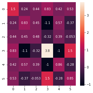
Positive Definite: Passed
Positive Semi-Definite: Passed
Symmetric: Passed
Positive Determinant: Passed
Eigen Values, Positivity: Passed

Test 2: Failure on Eigen Positivity

This test takes the complete breast cancer dataset and it failes for Eigen Positivity. This could be due to error in data entry, duplicate input or multiple entries. This gives an indicator to work on various front from cleaning the data to building better model. Though we did not build any models here, the matrix as such is pushing us to a progressive path.

cov = np.cov(bc_df, bias=True)
results = covariance_test(cov, (4, 0))
print_results(results)

Positive Definite: Passed
Positive Semi-Definite: Passed
Symmetric: Passed
Positive Determinant: Passed
Eigen Values, Positivity: Failed

Test 3: Failure on Multiple Fronts

In this case a subset was taken from the top right corner of the dataset and it fails at two counts

• Positive Determinant
• Eigen Positivity

cov = np.cov(bc_df[0:15, 20:25], bias=True)
results = covariance_test(cov, (4, 0))
print_results(results)

Positive Definite: Passed
Positive Semi-Definite: Passed
Symmetric: Passed
Positive Determinant: Failed
Eigen Values, Positivity: Failed

Inference

In this post we analyzed the properties of a covariance matrix - both geometrically and statistically. We also proved the positive semi-definite property of a matrix through covariance matrix computation formula. Subsequently, we tested the UCI Breast Cancer Dataset for the properties and inferred the significance. This will naturally lead to examine the following topics,

• Eigen values, vectors and spaces: One of my favorite topics
• Convex Optimization
• Gradient descent, especially stochastic gradient descent etc

References

• Math 2270 - Lecture 33 : Positive Definite Matrices by Dylan Zwick
• Math Help Boards: proof that covariance matrix is positive semidefinite
• What is the proof that covariance matrices are always semi-definite?
• Positive Definite Matrices
• Properties of the Covariance Matrix
• Covariance and Correlation
• Is a sample covariance matrix always symmetric and positive definite?
• Breast Cancer Wisconsin (Diagnostic) Data Set