Trend, Features of Structural Time Series, Mathematical Intuition Behind Trend Analysis for STS
Posted August 14, 2021 by Gowri Shankar ‐ 6 min read
Decomposability is the prime factor for the success of Generalized Additive Models in the quest for forecasting future events from the observed dataset. When we design a time series forecasting model, the functional features that we often observe from the data are trend, seasonality and impact points. The decomposable nature of these features from the dataset makes the problem conducive to model individual features independently by considering it as a curve fitting exercise. i.e. Modeling trend independently from other features makes the outcomes interpretable and subsequently paves way for advantages like bringing analyst in the loop in attaining convergence. This approach ignores the explicit dependence of temporal structure in the data that is a common function in generative models like ARIMA.
This is the 3rd post on STS and GAMs for time series forecasting, in our second post we studied seasonality as a harmonic sin and cosinusoids using Fourier analysis. In this post, we study trend on two counts,
- A Nonlinear, Saturating Growth and
- A Piecewise Logistic Model
Refer other posts in this series here,
- Fourier Series as a Function of Approximation for Seasonality Modeling - Exploring Facebook Prophet’s Architecture
- Structural Time Series Models, Why We Call It Structural? A Bayesian Scheme For Time Series Forecasting
- Is Covid Crisis Lead to Prosperity - Causal Inference from a Counterfactual World Using Facebook Prophet

Objectives
Our objective is to understand the mathematical intuition behind Nonlinear Growth and Piecewise Logistic Growth models. In that quest, we will be learning the following,
- Why we call it a saturating model
- Math behing Linear, Logistic and Exponential growth models
- Shape of the observation and selection of a model
- What is carrying capacity?
- What are piecewise models and when we use them
Introduction
English dictionary defines Trend as a general development or change in a situation or in the way that people are behaving. In the context of machine learning, It is a model trying to fit the data into a straight line - Yes, It is as simple as that. In the scheme of fitting the data to a straight, trend methods determines the speed and direction of any given entity’s progression(growth or fall). We infer the slope of the fitted line as direction of the trend(upward/downward) and the rate at which the movement happens is the speed. Growth is non-linear and saturates when it attains it’s carrying capacity, hence we often see fluctuations and then change in direction - We call it period of volatility and usually a flip in the direction of the progression(upward to downward and vice versa).
Saturating Growth Model
In this section, we shall build the mathematical intuition behind a growth model by understanding linear growth and logistic growth.
Linear Growth Model
We have to understand why we call it a saturating growth model and what exactly saturating. Given a data sequence $((x_1, y_1), (x_2, y_2), (x_3, y_3), \cdots, (x_n, y_n))$ the equation of a saturation growth function $f(x)$ is
$$\Large f(x) = y = a . \frac{x}{b + x} \tag{1. Saturation Growth}$$
$$f(x) = \displaystyle{\lim_{x \to \infty}} a . \frac{x}{b + x}$$
$$f(x) = \displaystyle{\lim_{x \to \infty}} a . \frac{x}{b/x + 1}$$
$$i.e$$
$$\Large f(0) = 0, f(\infty) = a \tag{2. Saturates at a}$$
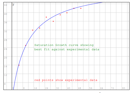
Growth saturation approximately looks as below,

- Image Credit - Non-Linear Regression - Saturation Growth Curve by The Enviro Engineer
With some clever math through substitution of the $eqn.1$, we can get the form of a linear model. i.e. take inverse transform of $eqn.1$
$$\Large \frac{1}{y} = \frac{b + x}{ax}$$
$$i.e.$$
 $$then$$
$$\Large z = a_0 + a_1.w \tag{3. Linear Model}$$
Our goal is to figure out $(a, b)$ and we know how to solve for $(a_0, a_1)$ by inverting $(x_i, y_i)$ $$z_i = \frac{1}{y_i}, i= 1, \cdots, n$$ $$w_i = \frac{1}{x_i}, i= 1, \cdots, n$$ $$then$$ $$\Large a = \frac{1}{a_0}, \ b = a_1a = \frac{a_1}{a_0} \tag{4. Solving a and b}$$
Nonlinear, Logistic Growth Model
A linear growth model is intuitive for our comprehension but not sufficient for convergence, also to account the non-linearity of its environment we extend it to a logistic growth model - for e.g. a product’s sale in a particular locality is function of the purchasing power of its residents. Purchasing power is the carrying capacity of the locality and sales growth saturates when it achieves its capacity.

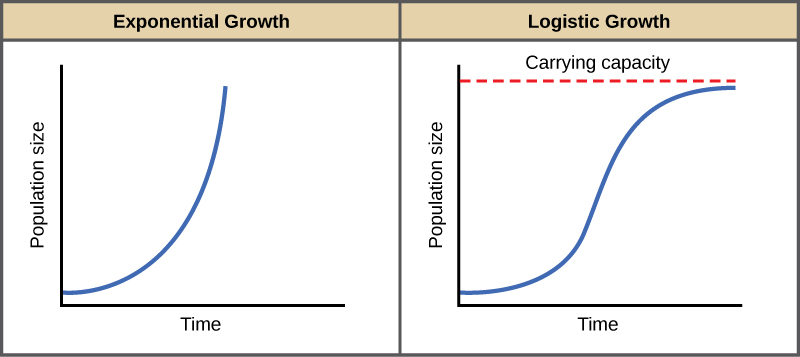
- Image Credit: Biology - Environment Limit to Population Growth
When resources are unlimited, populations exhibit exponential growth, resulting in a J-shaped curve.
When resources are limited, populations exhibit logistic growth. In logistic growth, population
expansion decreases as resources become scarce, and it levels off when the carrying capacity of
the environment is reached, resulting in an S-shaped curve.
- OpenStax, Biology
A logistic growth model can be written as
$$g(t) = \frac{C}{1 + e^{(-k(t-m))}} \tag{5. Logistic Growth Model}$$
Where,
- $C$ is the carrying capacity
- $k$ is the growth rate
- $m$ is the midpoint of the sigmoid
When we account the varying capacity which is a function of time, the equation evolves as below $$\Large g(t) = \frac{C_t}{1 + e^{(-k(t-m))}} \tag{6. Time Varying Logistic Growth Model}$$
The kind of model selection can be easily identified by observing the curve the dataset exhibits,
- Linear - An
inverted J-Shape - Logistic - An
S-Shape - Exponential - A
J-Shape
Piecewise Logistic Growth
If we closely examine the $eqn.6$, the growth rate is considered as a constant and it is a fallacy because environmental stimuli inherently alters the rate of growth. This phenomenon of change in growth is accounted by defining changepoints($S$) at times $s_j$. Let us say our base rate is $k$ and we have a vector of rate adjustments $\delta$, i.e the rate at any given time $t$ is $$k + \sum_{j:t > s_j} \delta_j$$ $$i.e$$ $$a(t) \in {0, 1}^S$$ $$then$$ $$\Large k + a(t)^T\delta \tag{7. Adjusted Growth Rate}$$ Since the growth rate is adjusted, the midpoint of the sigmoid $m$ has to be adjusted $$\gamma_j = \left(s_j - m \sum_{l < k} \gamma_l\right)\left(1 - \frac{k + \sum_{l < j}\delta_l}{k + \sum_{l \leq j}\delta_l}\right) \tag{8. Adjusted Sigmoid Midpoint}$$ $$Applying \ the \ adjustments \ to \ eqn.6$$
$$\Large g(t) = \frac{C_t}{1 + e^{(-(k + a(t)^T\delta)(t-(m + a(t)^T\gamma))}} \tag{9. Piecewise Logistic Growth Model}$$
Analyst in the Loop
$eqn.9$ accounts all challenging aspects of building a forecast models - It also exposes interfaces for an expert to bring in his domain knowledge. Let us examine few interesting aspects from our study and the equations we have derived,
- $C_t$ the time varying capacity can be set by an expert, Analysts often have insights of market dynamics and impact factors that could affect the outcomes significantly
- $s_j$ the changepoints can be specified by the analyst based on impact factors and events of significance
- When changepoints are not required, piecewise growth can be reduced to standard one by controlling $\delta$ and $\gamma$ values
Conclusion
This post explores the Trend feature of a time series model under GAMs family, we studied linear growth and derived the mathematical intuition behind it. Subsequently, we built a logistic growth model by discussing the drawbacks of a linear model. We discussed capacity saturations and situations when exponential growth has to be considered. At the end, we built a piecewise logistic modeling framework accounting time varying capacity and sigmoid midpoints. This post along with the previous 2 posts created a strong platform for us to venture into topics like uncertainty in a time series setup and much more. Hope you enjoyed this short read - Signing off for now.
References
- Non-Linear Regression - Saturation Growth Curve by The Enviro Engineer
- Forecasting at scale by Sean Taylor and Benjamin Latham of Facebook, 2017
- Nonlinear Regression by Autar Kaw
- Tend Methods using Mathematics from WW2010 University of Illinois
- Biology: Environmental Limits to Population Growth from OpenStax Biology
- Logistic Growth Model - Fitting a Logistic Model to Data, II by Leonard Lipkin and David Smith from Mathematical Association of America 2001