Story Behind

It’s the job that’s never started as takes longest to finish. - Samwise Gamgee

Of late I noticed my folks are struggling on performance optimization while building a high throughput machine for a mission critical application. This notebook might give some idea on how to approach compute complexity and avoid obvious bottlenecks in an abstract fashion.

There is a good chance one might seek an external reference to comprehend this notebook fully.

Disclaimers

• Cases are presented in abstraction
• Intent is to avoid disputes due to comparison of entities, operations and ideas
• Concrete examples are given but at algebraic level for human comprehension
• Artefacts like databases, storage and compute are not spoken - Concrete Entities
• Limitations of relational storage, indexing of labels for optimized retrievals are not spoken - Concrete Operations
• Which is better, SQL or NoSQL or Maps and Reduces etc are not spoken - Concrete Ideas

Rules

All we have to decide is what to do with the time that is given to us - Gandalf the Grey

5 rules to share the lifetime,

2 says what to be omitted,

3 says what grows faster,

and they all govern the time given to us.

They are

• Multiplicative Constants can be omitted
• Out of 2 polynomials, one with larger degree grows faster
• Any polynomial grows slower than any exponential
• Any polyalgorithm grows slower than any polynomial
• Smaller terms can be omitted

Big-O Notations

Intent of this notebook is to explore briefly the computation complexity through polynomial functions and

• Visualize the order of growth of frequently used functions in the algorithmic analysis
• Interactive(Using Jupyter Notebook) to play around with it
• Plug in your function of choice

Definitions

• Consider 2 functions f(n) and g(n) that defined for all positive integers and take on non-negative values
• Frequently used functions:
  \begin{equation*} log(n) \ sqrt(n) \ n log(n) \ n^3 \ 2^n \ \end{equation*}
• Let us say, f grows slower than g and f < g. ie f(n)/g(n) -> 0 as n grows
• f grows no faster than g, f <= g. ie for all n \begin{equation*} f(n) ⪯ c.g(n) \end{equation*}

Remarks

One

• f < g is same as f = o(g) and f<= g is same as f = O(g)
• Confusion 5n^2 = O(n^3) ie 5n^2 grows no faster than n^2 and slower than O(n^3)
• ie 5n^2 <= n^2 and 5n^2 <= n^3

Two

• If f < g, f ⪯ g. Lol if f grows slower than g, f certainly grows no faster than g

Three

• Symbol is ⪯ not ≤ because it is fancy

%matplotlib inline
import matplotlib.pyplot as plt
import numpy as np

Introduction: Growth of a Polynomial Function

It is not the strength of the body, but the strength of the spirit. - J.R.R. Tolkien

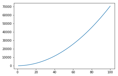
• Growth of a second order ploymial function or a quadratic equation with 3 coefficients.
• Plot is rendered on a larger space of 100 observations \begin{equation*} f(n) = 7n^2 + 6n + 5 \end{equation*}

n = np.linspace(1, 100)
plt.plot(n, 7*n*n + 6*n + 5)
plt.show()

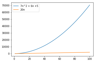
Compare a 2nd and 1st order function

• Growth is observed in a large space of 100 observations
• Difference is huge and the 1st order equation looks almost flat
• Graph is deceiving us \begin{equation*} f(n) = 7n^2 + 6n + 5 \ vs \ f(n) = 20n \ \end{equation*}

plt.plot(n, 7*n*n + 6*n + 5, label="7n^2 + 6n +5")
plt.plot(n, 20 * n, label="20n")
plt.legend(loc="upper left")
plt.show()

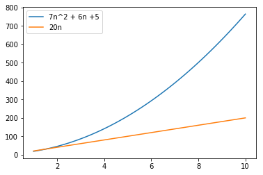
• Growth is observed for 1st order equation in the smaller space of 10 observations
• Difference is significant and the 1st order equation growth is not looking bad

n = np.linspace(1, 10)
plt.plot(n, 7*n*n + 6*n + 5, label="7n^2 + 6n +5")
plt.plot(n, 20 * n, label="20n")
plt.legend(loc="upper left")
plt.show()

Definitions: 5 Rules

A hunted man sometimes wearies of distrust and longs for friendship. - Aragorn

Common rules of comparing the order of growth of functions - Arising frequently in Algorithm Analysis
RULE 1: Multiplicative Constants can be omitted
for example ,
\begin{equation*} c.f ⪯ f \ \end{equation*} examples \begin{equation*} 5n^2 ⪯ n^2 \ n^2/3 ⪯ n^2 \ \end{equation*}

RULE 2: Out of 2 polynomials, one with larger degree grows faster
\begin{equation*} n^a⪯n^b \ for \ 0≤a≤b \ \end{equation*} Examples: \begin{equation*} n≺n^2 \ \sqrt{n}≺n^2/3 \ n^2≺n^3 \ n^0≺\sqrt{n}
\end{equation*}

RULE 3: Any polynomial grows slower than any exponential \begin{equation*} n^a≺b^n \ for \ a≥0 \ b>1 \end{equation*} Examples: \begin{equation*} n^3≺2^n \ n^{10}≺1.1^n
\end{equation*}

RULE 4: Any polyalgorithm grows slower than any polynomial
\begin{equation*} logn^a≺n^b \ for \ a,b>0 \end{equation*}

Examples:
\begin{equation*} logn^3≺\sqrt{n} \ nlogn≺n^2
\end{equation*}
RULE 5: Smaller terms can be omitted \begin{equation*} if \ f≺g \ then \ f+g⪯g \end{equation*}

Examples:
\begin{equation*} n^2+n⪯n^2 \ 2^n+n^9⪯2^n \end{equation*}

RULE 5: Smaller terms can be omitted

It is a strange fate that we should suffer so much fear and doubt over so small a thing… such a little thing. - Boromir

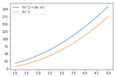
Let us take the RULE 5 first and analyse because it is simple and significant

• Growth is observed in a small space of 5 observations
• Difference is insignificant between the 2 equations
• Smaller terms 1st order and constant is ignored \begin{equation*} f(n) = 7n^2 + 6n + 5 \ vs \ f(n) = 7n^2 \ \end{equation*}

n = np.linspace(1, 5)
plt.plot(n, 7*n*n + 6*n + 5, label="7n^2 + 6n +5")
plt.plot(n, 7*n*n , label="7n^2")
plt.legend(loc="upper left")
plt.show()

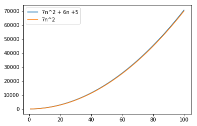
In a larger space of 100 observations they are almost same. Hence the significance of smaller terms are almost none.

n = np.linspace(1, 100)
plt.plot(n, 7*n*n + 6*n + 5, label="7n^2 + 6n +5")
plt.plot(n, 7*n*n , label="7n^2")
plt.legend(loc="upper left")
plt.show()

RULE 1: Multiplicative Constants Can Be Omitted

Torment in the dark was the danger that I feared, and it did not hold me back. - Gimli

With the same polynomial equation . \begin{equation*} 7n^2 + 6n + 5 = O(n^2) \end{equation*}

• lhs grows no faster than n^2
• ie Coefficient 7 for the second order item is insignificant

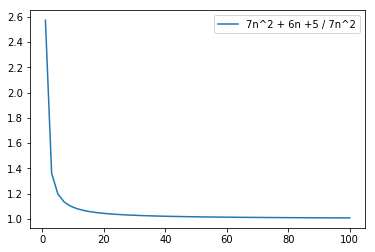
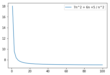
Same function with a different perspective
For absolute amusement let us demonstrate this rule with negative growth. ie \begin{equation*} f(n) = \frac{7n^2 + 6n + 5}{7n^2} \ vs \ f(n) = \frac{7n^2 + 6n + 5}{n^2} \ \end{equation*}

plt.plot(n, (7 * n * n + 6 * n + 5)/(7 * n * n), label="7n^2 + 6n +5 / 7n^2")
plt.legend(loc="upper right")
plt.show()

plt.plot(n, (7 * n * n + 6 * n + 5)/(n * n), label="7n^2 + 6n +5 / n^2")
plt.legend(loc="upper right")
plt.show()

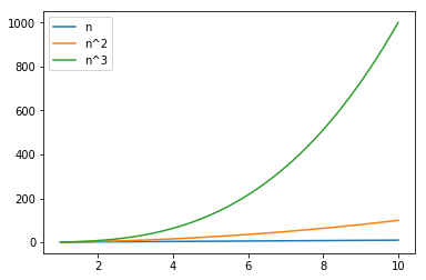
RULE 2: Out of 2 polynomials, the one with larger degree grows faster

Maybe the paths that you each shall tread are already laid before your feet, though you do not see them. - Lady Galadriel

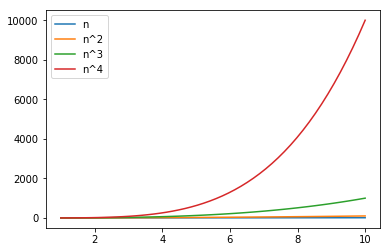
This is one another obvious item in the list of our rules ie \begin{equation*} n ≺ n^2 ≺ n^3 ≺ n^4 \end{equation*}

In a smaller space comparison of first 3 orders of the growth

n = np.linspace(1, 10)
plt.plot(n, n, label="n")
plt.plot(n, n * n, label="n^2")
plt.plot(n, n * n * n, label="n^3")
plt.legend(loc='upper left')
plt.show()

Upto 4th order in a smaller space

n = np.linspace(1, 10)
plt.plot(n, n, label="n")
plt.plot(n, n * n, label="n^2")
plt.plot(n, n * n * n, label="n^3")
plt.plot(n, n * n * n * n, label="n^4")
plt.legend(loc='upper left')
plt.show()

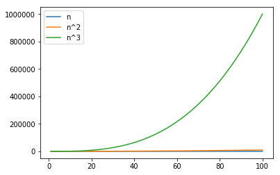
• In a larger space of 100 observations, 3rd order makes its predecessors looks so insignificant
• Needless to demostrate the 4th order

n = np.linspace(1, 100)
plt.plot(n, n, label="n")
plt.plot(n, n * n, label="n^2")
plt.plot(n, n * n * n, label="n^3")
#plt.plot(n, n * n * n * n, label="n^4")
plt.legend(loc='upper left')
plt.show()

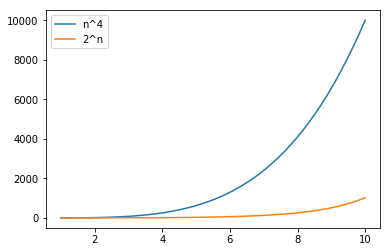
RULE 3: Any Polynomial grows Slower than Any Exponential

Why was I chosen?’ ‘Such questions cannot be answered - Gandalf the Grey

The most deceiving rule is this. One need to observe with a Million X zoom to really catch the critical section of transition. ie \begin{equation*} n^4 ≺ 2^n \ n^3 ≺ 2^n \end{equation*}

In a smaller space of 10 observation, It is observed \begin{equation*} 2^n ≺ n^4 \end{equation*}

n = np.linspace(1, 10)
plt.plot(n, n ** 4, label="n^4")
plt.plot(n, 2 ** n, label="2^n")
plt.legend(loc='upper left')
plt.show()

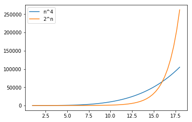
However n^4 is always greater than 2^n. In a different scale of 18 observations \begin{equation*} 1≤n≤18 \end{equation*} Exponential takes over at the point of intersection at 16th observeration. ie \begin{equation*} 2^4 = 4^2 \end{equation*}

n = np.linspace(1, 18)
plt.plot(n, n ** 4, label="n^4")
plt.plot(n, 2 ** n, label="2^n")
plt.legend(loc='upper left')
plt.show()

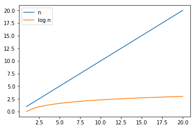
RULE 4: Any Polyalgorithm grows Slower than Any Polynomial

But in the end it’s only a passing thing, this shadow; even darkness must pass. - Samwise Gamgee

Growth of a logrithmic function is always slower than a polynomial \begin{equation*} log{(n)}≺n \ for \ a,b>0 \end{equation*}

n = np.linspace(1, 20)
plt.plot(n, n, label="n")
plt.plot(n, np.log(n), label="log n")
plt.legend(loc='upper left')
plt.show()

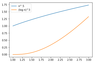
Square Root vs Log

$n^{0.5}$ vs $(\log n)^3$

It is useless to meet revenge with revenge: it will heal nothing - Frodo Baggins

A mind boggling and exotic example of square root versus logarithm: \begin{equation*} (\log n)^3 \ vs \ \sqrt{n} \end{equation*} (recall that $\sqrt{n}$ is a polynomial function since $\sqrt{n}=n^{0.5}$).

In a smaller space of 3 observations, proved \begin{equation*} (\log n)^3 ≺ \sqrt{n} \end{equation*}

n = np.linspace(1, 3)
plt.plot(n, n ** .5, label="n^.5")
plt.plot(n, np.log(n) ** 3, label="(log n)^3")
plt.legend(loc='upper left')
plt.show()

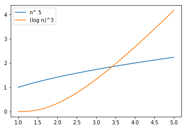
With 5 observations, extremely deceiving

\begin{equation*} (\log n)^3 > \sqrt{n} \end{equation*}

n = np.linspace(1, 5)
plt.plot(n, n ** .5, label="n^.5")
plt.plot(n, np.log(n) ** 3, label="(log n)^3")
plt.legend(loc='upper left')
plt.show()

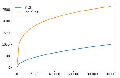
On a larger space of million observations, truth is questioned

n = np.linspace(1, 10**6)
plt.plot(n, n ** .5, label="n^.5")
plt.plot(n, np.log(n) ** 3, label="(log n)^3")
plt.legend(loc='upper left')
plt.show()

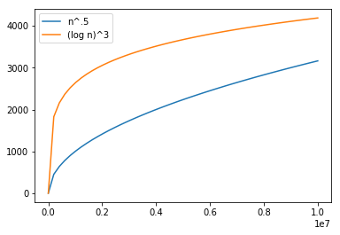
Truth is questioned even at 10s of million observation but there is some hope of convergence in the graph

n = np.linspace(1, 10**7)
plt.plot(n, n ** .5, label="n^.5")
plt.plot(n, np.log(n) ** 3, label="(log n)^3")
plt.legend(loc='upper left')
plt.show()

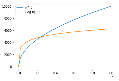
Truth prevails, when we pushed the limit to almost a billion observations

n = np.linspace(1, 10**8)
plt.plot(n, n ** .5, label="n^.5")
plt.plot(n, np.log(n) ** 3, label="(log n)^3")
plt.legend(loc='upper left')
plt.show()

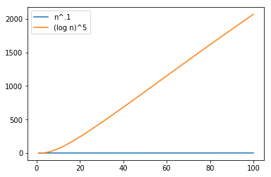
Fraction vs Log

$n^{0.1}$ vs $(\log n)^5$

Faithless is he that says farewell when the road darkens. - Gimli

Another sample where one can ponder the beauty of nature

At 100 Observations

n = np.linspace(1, 100)
plt.plot(n, n ** .1, label="n^.1")
plt.plot(n, np.log(n) ** 5, label="(log n)^5")
plt.legend(loc='upper left')
plt.show()

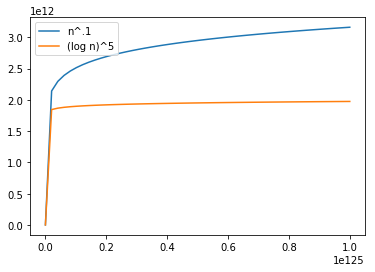
At 10^125 Observations: Truth Prevails

n = np.linspace(1, 10**125)
plt.plot(n, n ** .1, label="n^.1")
plt.plot(n, np.log(n) ** 5, label="(log n)^5")
plt.legend(loc='upper left')
plt.show()

Inference

Courage is the best defense that you have now - Gandalf the White

Through various polynomial functions we demonstrated the limiting behaviour of a function with different sets of arguments and observations space. This analysis should be foundation for arriving at running time or space requirement while designing a complex data centric operations. By merely expressing the ideas with an arithmatic function, one could understand the larger picture rather than focusing on smalling things.