That Straight Line Looks a Bit Silly - Let Us Approximate A Sine Wave Using UAT
Posted November 29, 2021 by Gowri Shankar ‐ 4 min read
This is the continuation of my first post on the Universal Approximation Theorem. My previous post took a simple case of approximating a leading straight line and in this post, we are approximating a sinewave using numpy that is smoothed using a Gaussian Filter.
Please consider this article an annex for the previous post, I added a few anecdotes from various personalities to make it look a bit interesting. Please read my previous posts before reading this article for clarity. This post comes under the subtopic Convergence under Math for AI/ML section. Please refer to the previous posts here
- Do You Know We Can Approximate Any Continuous Function With A Single Hidden Layer Neural Network - A Visual Guide
- Deep Learning is Not As Impressive As you Think, It’s Mere Interpolation
- Mathematics for AI/ML - Convergence

The key point in the Universal Approximation Theorem is that instead
of creating complex mathematical relationships between the input and
output, it uses simple linear manipulations to divvy up the complicated
function into many small, less complicated pieces, each of which are
taken by one neuron.

- Andre Ye
Objective
The objective of this article is to create a visual demonstration of approximating a sinewave in the 1-dimensional space.
Prologue
This post has 5 Sections that helps us to demonstrate the elegance of Universal Approximation Theorem by approximating a Sinewave
- Single Neuron
- Sine Wave Generator
- Series of Step Functions
- Tail Function
Single Neuron

- Image Credits: Artificial Neural Networks in a Nutshell

- Image Credit: Modeling Course Achievements of Elementary Education Teacher Candidates with Artificial Neural Networks
import numpy as np
import matplotlib.pyplot as plt

def neuron(inputt, weight, bias):
    f = lambda a, w, b: w * a + b
    step = lambda a, T: T if a >= T else 0

    f_of_x = f(inputt, weight, bias)
    output = [step(an_item, T) for an_item in f_of_x]

    return f_of_x, output

# Help functions to plot the graphs
def plot_steps(inputt, f_of_x, output, color, ax, title, label):
    ax.plot(inputt, f_of_x, color="green", label=f"f(x) = $\sum_i w_i x_i + bias$")
    ax.step(inputt, output, color=color, alpha=0.8, label=label)
    ax.set_title(title)
    ax.legend()
    ax.grid(True, which='both')
    ax.axhline(y=0, color='black', linewidth=4, linestyle="--")
    ax.axvline(x=0, color='black', linewidth=4, linestyle="--")

import matplotlib.image as mpimg
def render_image(ax, image_file):
    img = mpimg.imread(image_file)
    ax.imshow(img)
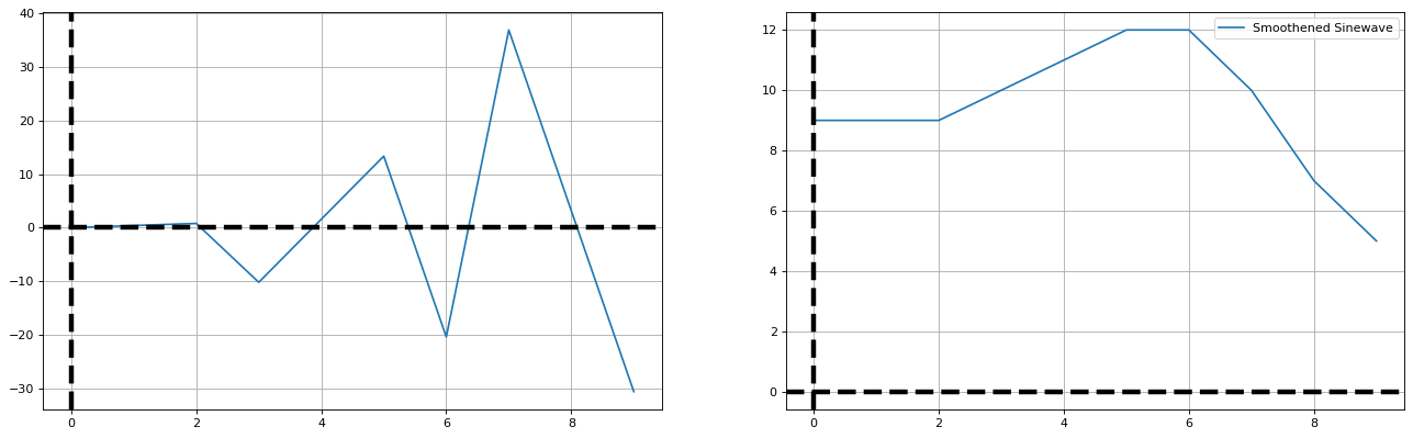
Sine Wave Generator
A sine wave is a geometric waveform that oscillates (moves up, down or
side-to-side) periodically, and is defined by the function y = sin x.
In other words, it is an s-shaped, smooth wave that oscillates above
and below zero.

- Adam Hayes

- Image Credit: Sinusoidal Wave Signal
# This code is written inspired by a stackoverflow post
# https://stackoverflow.com/questions/48043004/how-do-i-generate-a-sine-wave-using-python
from scipy.ndimage.filters import gaussian_filter1d

start_time = 0
end_time = 1
sample_rate = 10
time = np.arange(0, 10, 1)
theta = 0
frequency = 100
amplitude = 1
sinewave = amplitude * np.sin(2 * np.pi * frequency * time + theta) / 1e-14
_, axes = plt.subplots(1, 2, figsize=(20, 6), dpi=80)
axes[0].plot(sinewave, label="Sinewave")
smooth_sine = gaussian_filter1d(sinewave, sigma=2)
smooth_sine = np.array([round(item) + 10 for item in smooth_sine])
axes[1].plot(smooth_sine, label="Smoothened Sinewave")
plt.legend()
axes[0].grid(True, which='both')
axes[0].axhline(y=0, color='black', linewidth=4, linestyle="--")
axes[0].axvline(x=0, color='black', linewidth=4, linestyle="--")
axes[1].grid(True, which='both')
axes[1].axhline(y=0, color='black', linewidth=4, linestyle="--")
axes[1].axvline(x=0, color='black', linewidth=4, linestyle="--")
<matplotlib.lines.Line2D at 0x7f8adaf47970>
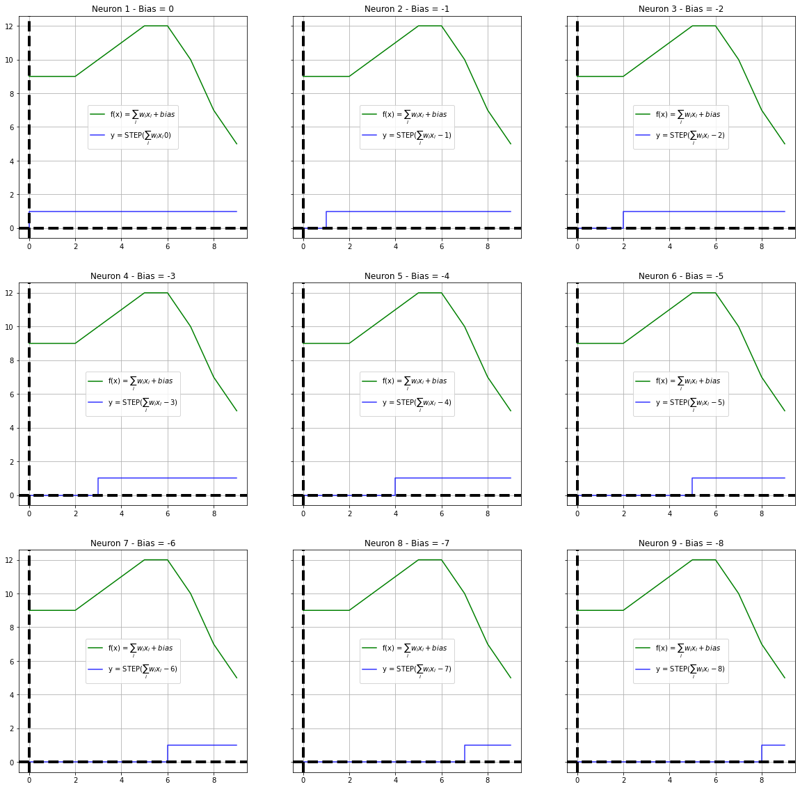
Simulating Series of Steps
We are creating 9 neurons in the the hidden layer and approximating the sinewave.
x = np.arange(10)
w = 1
T = 1
y = smooth_sine
fig, axes = plt.subplots(3, 3, figsize=(20, 20), sharey=True)
bias = -x
col = 0
row = 0
steps = []
for idx in np.arange(10):
    b = bias[idx]

    if col == 3:
        row += 1
        col = 0


    _, gx = neuron(x, w, b)
    steps.append(gx)
    if((col != 3) and (row != 3)):
        plot_steps(x, y, steps[idx], "blue", axes[row, col], f"Neuron {idx + 1} - Bias = {b}", label=f"y = STEP($\sum_i w_i x_i {b}$)")
    col += 1
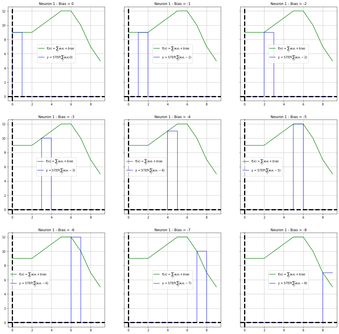
Tail Function
fig, axes = plt.subplots(3, 3, figsize=(20, 20), sharey=True)
bias = -x
print (axes.shape, x, bias)
col = 0
row = 0
tails = []
for idx in np.arange(9):
    b = bias[idx]
    tail = list(y[idx] * (np.array(steps[idx]) - np.array(steps[idx + 1])))
    tails.append(np.array(list(y[idx] * (np.array(steps[idx]) - np.array(steps[idx + 1])))))

    if col == 3:
        row += 1
        col = 0
    plot_steps(x, y, tail, "blue", axes[row, col], f"Neuron 1 - Bias = {b}", label=f"y = STEP($\sum_i w_i x_i {b}$)")
    col += 1
(3, 3) [0 1 2 3 4 5 6 7 8 9] [ 0 -1 -2 -3 -4 -5 -6 -7 -8 -9]
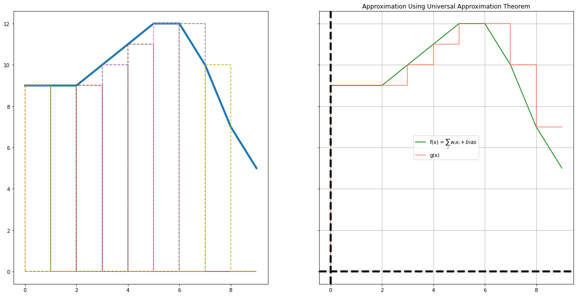
fig, axes = plt.subplots(1, 2, figsize=(20, 10), sharey=True)
bias = -x
axes[0].plot(x, y,linewidth=4)
for idx in np.arange(8):

    axes[0].step(x, tails[idx], linestyle="--")
gx = np.sum(tails, axis=0)
plot_steps(x, y, gx, "tomato", axes[1], title="Sum of Steps", label="g(x)")
plt.title("Approximation Using Universal Approximation Theorem")
Text(0.5, 1.0, 'Approximation Using Universal Approximation Theorem')
Epilogue
This is a continuation of the previous article on UAT inspired by Layra Ruis’ review on the paper Learning in High Dimension Always Amounts to Extrapolation. In this post, we approximated a sinusoidal wave using a neural network with 1 hidden layer. I am glad to present this topic, I had a few new learnings and hope my readers too. I thank everyone who inspired me to write this post, It is an amazing experience.