Survival Analysis using Lymphoma, Breast Cancer Dataset and A Practical Guide to Kaplan Meier Estimator
Posted November 20, 2021 by Gowri Shankar ‐ 9 min read
I live in the hills of Kumaon, the Himalayas a region of biodiversity, scenic beauty, and fertile landscapes situated to the west of Nepal. This region is full of fruit orchards that thrive due to the conducive condition and the fertile soil. An interesting aspect that caught my attention is the farmers allowing frugivores in their orchards to consume their produce that results in an effective seed-dispersing scheme. Most of the frugivores have a specialized digestive system to process fruits and leave the seeds intact from their gut. The quest is how long the farmers have to leave the fleshy fruits in their orchards so that the animals consume them for an effective seed-dispersing process. Statistics have the answer, Survival analysis is a methodology widely used in medical research to measure the probability of patients living after a certain amount of time after the treatment for a disease. It comes under the medical prognosis scheme of healthcare. Using survival analysis we can find how long the fleshy fruits have to remain in the tree for the frugivores to consume.
We do not have any significant data from the farmers having effective seed-dispersing through frugivores but we have abundant data for survival analysis from healthcare. In this post, we shall brief the fundamentals of survival analysis and develop Kaplan Meier Estimator from the scratch. This comes under the series Math for Machine Learning under the sub-section Statistics, please refer to the previous post in this series here

- Image Credit: Survival Analysis: Intuition & Implementation in Python
I thank Pranav Rajpurkar for his amazing course AI for Medicine Specialization in Coursera. This post is inspired by whatever he taught me on Medical diagnosis, prognosis and treatment. Without his quality work, I would’nt have written this post.
Objective
The key objective of this post is to understand the significance of Survival Analysis and develop Kaplan Meier Estimator from scratch without using any libraries.
Introduction
Time to an event - Survival Analysis is a statistical procedure through which we calculate the time taken for an event to occur after an intervention happened. Following are some of the examples of survival analysis,
- Time to death: Time taken for a patient to die after diagnosing HIV
- Time to consume: Time taken for a fleshy fruit to be eaten by a frugivore
- Time to malfunction: Time taken by an automobile to go immobile after identifying a faulty part
- Time to monetize: Time taken by a user to switch from a regular subscription to a premium subscription
- Time to contribute: Time taken by a Kaggle user to Kaggle contributor
The dataset for survival analysis consists of two key ingredients, a. whether an event occurs or not (1 - event occurred, 0 - the event did not occur) b. the follow-up time of observation ( duration at which monitoring and data collected)
Another important aspect of survival analysis is the event of interest occurs only once for a subject.
We can formalize the above ideas and represent the survival as a function where the probability of the event of interest not occurring by the time $t$. For example, what is the probability of death not occurring by the time $t$.
$$S(t) = P_r(T > t) \tag{1. Survival function}$$ Where,
- $P_r$ is the probability of an event not occurring
- $T$ is the time at which the event eventually occurred
- $t$ is the time at which the event did not occur(could be interpreted as follow up time)
The Hazard Function
Opposite of the survival function is the hazard function. i.e What if the event occurred within a short period after the specified period $t$. E.g. It has been observed Shaheen Shah Afridi of the Pakistani cricket team often takes his first wicket in his first over($t = 6 balls)$. Instead of scalping the opener in the first over, if he takes his first wicket on his $7^{th}$ ball (i.e. the first ball of his second over) then we call a hazard occurred. i.e the batsmen survived for 6 balls and a hazard occurred on the $7^{th}$ ball of Shaheen. $$\lambda(t) = \frac{P_r{t \leq T < dt | T \geq t}}{dt} \tag{2. Hazard Function}$$
Where,
- The numerator is the conditional probability of the event occurring given that it did not occur in the past.
- $dt$ is the duration of the considered period
then the ratio of the conditional probability of event occurrence to the considered period is nothing but the event occurrence per unit of time. Then the limit gives us a lens to the instantaneous rate of occurrence.
it is important to mention that the hazard function is not actually a probability and
the name hazard rate is the more fitting one. That is because even though the expression
in the numerator is the probability, the dt in the denominator can actually result in a
value of the hazard rate greater than 1 (it is still limited to 0 at the lower interval).

- Eryk Lewinson
The relationship between survival and hazard function is defined as follows $$S(t) = \Large e^{{-\int_0^t \lambda(x)dx}} \tag{3. Suvival Function in Terms of Cumulative Hazard}$$
Kaplan Meier Estimator
In this post, we shall study the Kaplan-Meier Estimator of survival analysis in detail. There are many statistical methods through which we can estimate the survival period and they are classified as follows,
- Non-parametric: without making any assumption about the underlying distribution of data, estimation is done. e.g. Kaplan-Meier Estimator
- Semi-parametric: few assumptions but there is no assumption about the shape of the hazard function. e.g. Cox Regression
- Parametric: By using statistical distributions to estimate maximum-likelihood(MLE). e.g. Weibull, Lomax etc
Kaplan-Meier estimator plots the survival probability as a function of time. We define this estimator as an approximation function as follows
$$S(t) = \prod_{t_i \leq t} (1 - \frac{d_i}{n_i}) \tag{4. Kaplan-Meier Estimator}$$
Where,
- $t_i$ are the time of event observed in the dataset
- $d_i$ is the number of events occurred at time $t_i$
- $n_i$ is the number of subjects who we know has survived up to time $t_i$.
Kaplan Meier Implementation
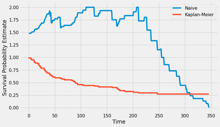
In this section, we shall implement two survival probability estimators and compare them
- A Naive Estimator and
- Kaplan-Meier Estimator as per the $eqn.4$
import numpy as np
import pandas as pd
import matplotlib.pyplot as plt

plt.style.use('fivethirtyeight')

def naive(t, df):
    return sum(df['Time'] > t) / sum(df['Event'] == 0 | (df['Time'] > t) )

def kaplan_meier(df):
    event_times = [0]
    p = 1.0
    S = [p]

    observed_event_times = df['Time'].unique()
    observed_event_times = np.sort(observed_event_times)

    for t in observed_event_times:
        num_survived_at_t = sum(df['Time'] >= t)
        num_failed_to_survive_at_t = sum((df['Time'] == t) & (df['Event'] == 1))

        p = p * (1 - num_failed_to_survive_at_t / num_survived_at_t )
        S.append(p)
        event_times.append(t)
    return event_times, S
Verify Kaplan-Meier Implementation using Lymphoma Dataset
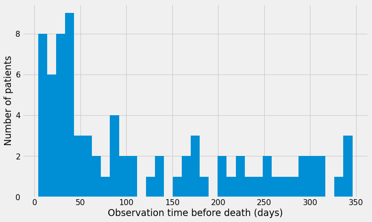
We shall load lymphoma data from the lifelines dataset and verify our implementation of the Kaplan-Meier estimator and Naive estimator. This dataset shows how many days a patient has survived since they were diagnosed with Lymphoma.
from lifelines.datasets import load_lymphoma

df_lymphoma = load_lymphoma()
df_lymphoma.loc[:, 'Event'] = df_lymphoma.Censor
df_lymphoma = df_lymphoma.drop(['Censor'], axis=1)

df_lymphoma.head()
| Stage_group | Time | Event | |
|---|---|---|---|
| 0 | 1 | 6 | 1 |
| 1 | 1 | 19 | 1 |
| 2 | 1 | 32 | 1 |
| 3 | 1 | 42 | 1 |
| 4 | 1 | 42 | 1 |
plt.figure(figsize=(10, 6), dpi=80)

df_lymphoma.Time.hist(bins=35);
plt.xlabel("Observation time before death (days)");
plt.ylabel("Number of patients");
x = range(0, df_lymphoma.Time.max() + 1)
y = np.zeros(len(x))

for i, t in enumerate(x):
    y[i] = naive(t, df_lymphoma)

plt.figure(figsize=(10, 6), dpi=80)
plt.plot(x, y, label='Naive')

x, y = kaplan_meier(df_lymphoma)
plt.step(x, y, label='Kaplan-Meier')
plt.xlabel('Time')
plt.ylabel('Survival Probability Estimate')
plt.legend()
plt.show()
Breast Cancer: Survival Analysis
In this section, we shall download Haberman’s Breast cancer survival data collected between 1958 and 1970 at the University of Chicago’s Billings Hospital. This data has the details of the patients who survived 5 years or longer and the patients who died within 5 years. To do survival analysis, I created synthetic data(random) for the “Time of Event” $t$ variable for those who died within 5 years.
Preprocessing and Exploration
Following are the steps involved in preprocessing section,
- Load the data using pandas package and store it as a Dataframe
- Explore the data
- Separate the data of the patients who died before 5 years
- Mark the patients who had more than 10 auxiliary nodes as Group 1 and the rest Group 2 for sub-group analysis
df_breast_cancer = pd.read_csv("haberman.csv", header=None)
df_breast_cancer.columns = ['Age','opYear','auxNode','Survival']
df_breast_cancer.Survival -= 1
df_breast_cancer.head()
| Age | opYear | auxNode | Survival | |
|---|---|---|---|---|
| 0 | 30 | 64 | 1 | 0 |
| 1 | 30 | 62 | 3 | 0 |
| 2 | 30 | 65 | 0 | 0 |
| 3 | 31 | 59 | 2 | 0 |
| 4 | 31 | 65 | 4 | 0 |
df_breast_cancer.Survival.value_counts() / len(df_breast_cancer)
0    0.735294
1    0.264706
Name: Survival, dtype: float64
According to this data, 75% of the patients survived at least 5 years after the surgery.
df_event_occurred = df_breast_cancer[df_breast_cancer["Survival"] == 1]
df_event_not_occurred = df_breast_cancer[df_breast_cancer["Survival"] == 0]
df_event_occurred.loc[:, "Time"] = np.random.choice(60, 81)
mask = df_event_occurred.auxNode > 10
df_event_occurred["Group"] = mask
df_event_occurred.head()
/Users/shankar/dev/tools/anaconda3/envs/od/lib/python3.8/site-packages/pandas/core/indexing.py:1597: SettingWithCopyWarning:
A value is trying to be set on a copy of a slice from a DataFrame.
Try using .loc[row_indexer,col_indexer] = value instead

See the caveats in the documentation: https://pandas.pydata.org/pandas-docs/stable/user_guide/indexing.html#returning-a-view-versus-a-copy
  self.obj[key] = value
/Users/shankar/dev/tools/anaconda3/envs/od/lib/python3.8/site-packages/pandas/core/indexing.py:1676: SettingWithCopyWarning:
A value is trying to be set on a copy of a slice from a DataFrame.
Try using .loc[row_indexer,col_indexer] = value instead

See the caveats in the documentation: https://pandas.pydata.org/pandas-docs/stable/user_guide/indexing.html#returning-a-view-versus-a-copy
  self._setitem_single_column(ilocs[0], value, pi)
<ipython-input-7-3cc733e02e76>:5: SettingWithCopyWarning:
A value is trying to be set on a copy of a slice from a DataFrame.
Try using .loc[row_indexer,col_indexer] = value instead

See the caveats in the documentation: https://pandas.pydata.org/pandas-docs/stable/user_guide/indexing.html#returning-a-view-versus-a-copy
  df_event_occurred["Group"] = mask
| Age | opYear | auxNode | Survival | Time | Group | |
|---|---|---|---|---|---|---|
| 7 | 34 | 59 | 0 | 1 | 55 | False |
| 8 | 34 | 66 | 9 | 1 | 14 | False |
| 24 | 38 | 69 | 21 | 1 | 24 | True |
| 34 | 39 | 66 | 0 | 1 | 22 | False |
| 43 | 41 | 60 | 23 | 1 | 23 | True |
df_event_not_occurred.shape, df_event_occurred.shape
((225, 4), (81, 6))
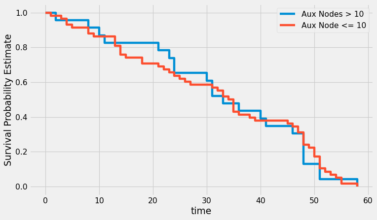
Sub-Group Analysis
Using Kaplan-Meier fitter from the lifelines package, we shall do the survival analysis and compare the group 1 patients with group 2 patients.
from lifelines import KaplanMeierFitter
from lifelines.statistics import logrank_test
df = df_event_occurred.copy()
group_1 = df[df["Group"] == True]
group_2 = df[df["Group"] == False]
km_grp_1 = KaplanMeierFitter()
km_grp_1.fit(group_1.loc[:, "Time"], event_observed=group_1.loc[:, "Survival"], label="Aux Nodes > 10")
km_grp_2 = KaplanMeierFitter()
km_grp_2.fit(group_2.loc[:, "Time"], event_observed=group_2.loc[:, "Survival"], label="Aux Node <= 10")
/Users/shankar/dev/tools/anaconda3/envs/od/lib/python3.8/site-packages/lifelines/fitters/kaplan_meier_fitter.py:351: FutureWarning: Support for multi-dimensional indexing (e.g. `obj[:, None]`) is deprecated and will be removed in a future version.  Convert to a numpy array before indexing instead.
  self.confidence_interval_ = self._bounds(cumulative_sq_[:, None], alpha, ci_labels)


<lifelines.KaplanMeierFitter:"Aux Node <= 10", fitted with 58 total observations, 0 right-censored observations>
plt.figure(figsize=(10, 6), dpi=80)
ax = km_grp_1.plot(ci_show=False)
km_grp_2.plot(ax=ax, ci_show=False)
plt.xlabel('time')
plt.ylabel('Survival Probability Estimate')
Text(0, 0.5, 'Survival Probability Estimate')
Log Rank Test
Log Rank Test is used to compare teh survival curves of two groups.
lr_result = logrank_test(group_1.Time, group_2.Time, group_1.Survival, group_2.Survival)
lr_result.__dict__
{'p_value': 0.9158306594818046,
 'test_statistic': 0.011169751451570351,
 'test_name': 'logrank_test',
 '_p_value': array([0.91583066]),
 '_test_statistic': array([0.01116975]),
 'name': None,
 't_0': -1,
 'null_distribution': 'chi squared',
 'degrees_of_freedom': 1,
 '_kwargs': {'t_0': -1,
  'null_distribution': 'chi squared',
  'degrees_of_freedom': 1,
  'test_name': 'logrank_test'}}
Conclusion
In this post, we studied survival analysis briefly and in that process, we built a Kaplan-Meier estimator without any sophisticated statistics packages. We also explored Lymphoma and Breast Cancer datasets in conducted a survival analysis. The purpose of this post is academic to learn whereas concepts in a practical setup concerning survival analysis, ie. our intention is not to conclude anything from the data. I am glad to start a series on Statistics for ML with an end-to-end implementation hope it helps the reader. Thank you.
References
- Haberman’s Survival Data Set by GilSousa
- Survival Analysis by Lisa Sullivan, Boston Univ
- Introduction to Survival Analysis: the Kaplan-Meier estimator by Eryk Lewinson, 2020
- Introduction to Survival Analysis by Eryk Lewinson, 2020
- Kaplan–Meier estimator from Wikipedia