Structural Time Series Models, Why We Call It Structural? A Bayesian Scheme For Time Series Forecasting
Posted August 1, 2021 by Gowri Shankar ‐ 7 min read
Models we build are the machines that has fundamental capability to learn the underlying patterns in the observed data and store them in the form of weights. Patterns reside in different forms, shapes and sizes - this is ubiquitous because we are interpreting the universe through our observed data. When the observed data exhibit periodic patterns - we call them time series. The key challenge with time series data is the missing values and absence of confounders - makes them special. Further the problem gets more interesting when we approach time series forecasting in a Bayesian setup. This is a new series of posts I am starting with Structural Time Series(STS) where we explore a wide gamut of problems and approaches to declutter the underlying treasure.
In this post, we shall introduce time series by studying the nature of the observations, foundational concepts with a focus on building probabilistic models. The novelty in this post is Bayesian but nothing much dealt now, left it for future posts. Time series posts are not completely new, We have studied time series models in the past under Model Explainability and Causal Inferencing from a Counterfactual world. Please refer,
- Is Covid Crisis Lead to Prosperity - Causal Inference from a Counterfactual World Using Facebook Prophet
- Higher Cognition through Inductive Bias, Out-of-Distribution and Biological Inspiration

- Image Credit: Introduction to Time Series Analysis in Machine learning
Objective
The main objective of this post is to understand why we call time series models as Structural Time Series Models, In this quest we study the following topics
- Generalized additive models
- State Space Models
- Latent Space Dynamics
- Classification of Time Series Models
- Functions of approximation for
Trend,SeasonalityandImpact
Introduction
I had the opportunity to work with sales data of quite a good number of Fast Moving Consumer Goods(FMCG) manufacturers across geographies and product categories(e.g. Personal/Fabric Care, Dairy Products, Bakery Products etc) - When it comes to sales forecasting, It is not a rocket science to start the research on beverage(If you have and I am lucky on this front to study alcoholic beverages) consumption data at national, regional and global level. It is often the trend is seen with respect to the weather patterns - a major confounder. i.e. Beer consumption goes uphill from winter to summer and falls during the other half of the year and an opposite pattern for spirits(e.g. Whiskey, Rum etc) consumption. Also, I have noticed no significant change in equatorial or tropical countries due to low temperate climate that are mostly tropical in nature.
Trivia: Time Dependent Confounders
Information like weather patterns, air pollution on a given day, body sugar level wrt food intake etc are time dependent confounders of diverse intervals.
Trivia: Confounders or Correlated
Periodic patterns like weather, food intake etc are often believed as correlated features but they are not. They are the confounders, studied as causal concept rather than an associated feature.
Trivia: Latent Space Dynamics
Though the term Latent Space Dynamics sounds quite fancy, It is nothing but the well known concept of embeddings. i.e We create a new feature space and project the variable values within a manifold in which items that resemble each other more are positioned closely to one another.
Most of the time series data displays the following characteristics,
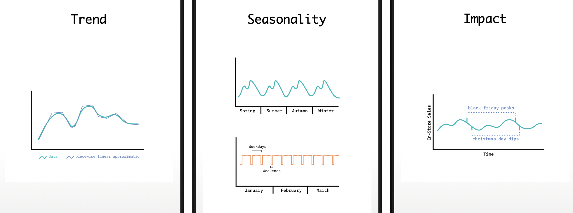
- Trend: General upward or downward trends, like beer consumption during the course of a year
- Seasonality: Repeating and nested patterns, like grocery purchases peaks during beginning of the month and nested peaks due to weekend shopping spree
- Impacts: Sudden spikes and drops in the observations due to impactful events, like festivals, black friday sale etc.
- Exogenous Variables: Fancy again, It is just external attributes that are not part of the observed data, e.g. Weather data.
$$observation(t) = trend(t) + seasonality(t) + impact(t) + noise$$
- Images Credit: Structural Time Series
Combination of these functions constitutes the characteristics of the observed data, similar to a linear mixed signals that we studied in Independent Component Analysis.
Classification of Structural Time Series
Foundation of Structural Time Series models are the linear mixing of various functions, mainly those that we have discussed earlier. Further, the models are classified into two,
- State Space Models(SSM) generated by Latent Space Dynamics and
- Generalized Additive Models(GAM) where time series is decomposed into functions that add together to reproduce the signals.
State Space Models
The well known ARIMA and Kalman Filters falls under the state space model category, where the time series is generated by latent space dynamics.
State space model(SSM) refers to a class of probabilistic graphical model(Daphne Koller et al) that
describes the probabilistic dependence between the latent state variable and the observed measurement.
...
SSM provides a general framework for analyzing deterministic and stochastic dynamical systems that are
measured or observed through stochastic process.

- Chen(MIT) and Brown(Harvard)
Generalized Additive Models
A generalized additive model is a generalized linear mixed model(GLM with additive mix) in which linear predictor depends linearly on unknown smooth functions of some of the predictor variables - focus is on the unknown smooth functions. This idea leads the time series problem as curve fitting one with interpretability, debug possibility and ablity to handle missing values along with irregular intervals of observed data. It provides a posterior distribution of forecasts that captures uncertainty.
Though both(SSM and GAM) the approaches falls under Bayesian class, the additive property of GAMs is an apt fit for a Structural Time Series due to it’s inherent nature of decomposability. For e.g. for a univariate time series data, the observed variable is decomposed into smooth function of time
- Trend
- Seasonality and
- Impact
Functions of Approximation
In this section, we shall study the nature of the 4 attributes and possible functions of approximation that helps us to design our modelling strategy. i.e We are defining a structure to our models through certain functions of approximation, hence Structural Time Series. On contrary an RNN can learn arbitrary functions.
Trend
Usually the time series observations shows upward or downward trend at larger intervals of time, if not often local trends are observed. A simple observation could be exponential growth(Covid outburst), then the modelling function could be a growing function of exponential kind. When the trend is more complex, a piecewise linear approximation function is proposed under smaller linear segments.
Logistic function is modeled when there is a saturation point. For e.g. A situation where covid spread is exponential but there is a limit in availability of hospital beds, health care workers and medical oxygen.
Seasonality
Seasonality is not just restricted to the natural phenomenon - anything periodic, that has a repeating pattern is seasonality. Underlying periodic patterns could have a daily cycle or weekly cycle or annual one - In a rare case, certain activities happen once in N number of years (some rare flower blooms once in 12 years. Few insects live just for a day and perish. To capture these phenomenons, we need a sophisticated function and Fouries Series comes to our rescue. Using Fourier Series, we can encode any periodic patterns,
A Fourier series is a weighted sum of sine and cosine terms with increasingly high frequencies. Including more
terms in the series increases the fidelity of the approximation. We can tune how flexible the periodic function
is by increasing the degree of the approximation (increasing the number of sine and cosine terms included).

- Fastforward Labs of Cloudera
The number of Fourier components is set by intuition or by brute hyperparameter search for convergence.
Impact
Impact effects are purely a matter of the expert’s discretion because they are not recurring patterns - A subject matter expert can identify these phenomenon and propose a scheme. For e.g. product promotion activities to boost the sales or effect of a holiday(christmas day sales dip) generally makes peaks and sharp trenches in the observed sequences. These discrete components are included as a constant term while modelling.
External Regressors
The three characteristics trend, seasonality and impact are strictly univariate - the only predictor is the observed variable over time. Since it is nothing but a curve fitting scheme of modelling, there is a provision to add more variables to the model.
There is only one challenge in adding external variables - If we want to forecast a value, we have to know what could be the possible value of the external variable of the future. That increases the complexity of our modelling scheme. For e.g. If weather is a confounder for beer sales, we can acquire weather data from meteorological agencies to add to our predictive models. A much sophisticated approach could be, we can predict the future values for various scenarios by simulating a corresponding exogenous data.
Inference
This is a quick refresher on the basics of time series modelling, we studied the nature of time series data in the context of generalized additive models. Subsequently, functions of approximation for key characteristics. In the future posts we shall extend our understanding by
- Studying the schemes of evaluating time series models
- Error functions like MAPE and MASE
- Autoregressive time series models
- A deeper study of Bayesian approach to time series etc
This is a quick and unmathy read that explores the underlying functions of a time series data, hope you all enjoyed it.