from IPython.display import Image

Forward and Backpropagation Algorithm

An associated source code will be published shortly.

In this post, we shall explore a shallow Dense Neural Network(DNN) with

• an Input Layer
• a Single Hidden Layer and
• an Output Layer

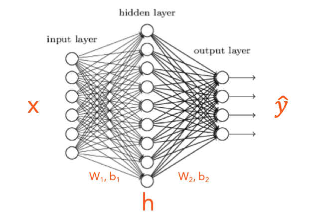
The typical architecture of a feed forward network has the above units. Where

• $x$ is a vector that represents the input values,
• $\hat y$ is a vector that represents the predictions and
• $h$ is vector that represents the hidden layer, $h$ is a hyperparameter selected based on the context of the problem

Further to the above 3 parameters, connection weights $[W_1, W_2]$ and connection biases $[b_1, b_2]$ are the other matrices and vectors used in a DNN

Architecture of a Shallow DNN

6 Inputs, 9 Hidden Nodes, 4 Outputs

display(Image("/kaggle/input/sample-images/shallow-dnn.png"))

Following are the processes we shall cover in the quest of understanding a simple Neural Network architecture,

• Forward Propagation
• Cross Entropy Loss (covered in a separate post)
• Activation Functions
  • Softmax
  • ReLU
• Backpropagation
• Gradient Descent
• Extraction of features of the hidden layer

From the above Diagram…

• There are 6 Inputs of dimension $(I \times 1)$ ie (6 X 1)
• There are 9 nodes in the Hidden Layer of dimension $(N \times 1)$ ie (9 X 1)
• There are 4 nodes in the Output Layer of dimension $(O \times 1)$ ie (4 X 1)

Forward Propagation

From the inputs and weights, biases of the hidden layer, $$z_1 = W_1x + b_1 \tag{1}$$ $$h = ReLU(z_1) \tag{2}$$ From hidden layer ($h$) and weights, biases to the output layer $$z_2 = W_2h + b_2 \tag{3}$$ $$\hat y = softmax(z_2) \tag{4}$$

Dimension Analysis

How to select the weights, let us do dimensionality reduction Let us examine the dimensions of all elements in the equation 1 $$z_1 = W_1h + b_1$$ $$dimensions$$ $$N \times 1 = [?, ?] \times [I, 1] + [?, ?]$$ $$naturally$$ $$N \times 1 = [N, I] \times [I, 1] + [N, 1]$$ $$hence$$ $$9 \times 1 = [9, 6] \times [6, 1] + [9, 1]$$ Hence $N \times I $ is the dimension of the weight matrix $W_1$

Let us examine the dimensions of all elements in the equation 2 $$z_2 = W_2h + b_2$$ $$dimensions$$ $$O \times 1 = [?, ?] \times [N, 1] + [?, ?]$$ $$then$$ $$O \times 1 = [O, N] \times [N, 1] + [O, 1]$$ $$hence$$ $$4 \times 1 = [4, 9] \times [9, 1] + [4, 1]$$ Hence $O \times N $ is the dimension of the weight matrix $W_2$

Cross Entropy Loss

Our goal is to minimize the loss $J$ $$J = - \sum\limits_{k=1}^V y_k \log\hat y_k \tag{5}$$ Cost(Loss) Function for Binary Classification - A Deep Dive

Backpropagation - Pull your sleeves and do some partial derivatives

We calculated the $\hat y$ during forward propagation and now our goal is to optimize the weights by minimizing the loss. This is done by calculating the partial derivatives wrt $[W_2, b_2]$ and then $[W_1, b_1]$ $$\frac{\partial J}{\partial W_1} = ReLU\left( W^T_2(\hat y - y)\right)x^T \tag{6}$$ $$\frac{\partial J}{\partial W_2} = (\hat y - y)h^T \tag{7}$$ $$\frac{\partial J}{\partial b_1} = ReLU\left(W^T_2(\hat y - y)\right) \tag{8}$$ $$\frac{\partial J}{\partial b_2} = \hat y - y \tag{9}$$

Gradient Descent

Gradient descent is the process during which the weights and biases are updated by subtracting $\alpha$ times the learning rate of calculated gradients from the original matrices and biases

$$W_1 := W_1 - \alpha\frac{\partial J}{\partial {W_{1}}} \tag{10}$$ $$W_2 := W_2 - \alpha\frac{\partial J}{\partial W_2} \tag{11}$$ $$b_1 := b_1 - \alpha\frac{\partial J}{\partial b_1} \tag{12}$$ $$b_2 := b_2 - \alpha\frac{\partial J}{\partial b_2} \tag{13}$$

Demystifying Gradient Descent - A Deep Dive