In-silico neuromorphism or neuromorphic computing is an interdisciplinary area of research bringing the best of biology, physics, mathematics, computer science and electronic engineering into a VLSI system that mimic(may not completely) the neuro-biological architecture of the nervous system. We studied and simulated spiking neurons, post-synaptic depression models in our earlier posts. Please refer,

• With 20 Watts, We Built Cultures and Civilizations - Story of a Spiking Neuron
• Understanding Post-Synaptic Depression through Tsodyks-Markram Model by Solving Ordinary Differential Equation

• Image Credit: Clinic Pain Advisor

In the past, in one of our posts we also built a transfer learning classification model for detecting Diabetic Retinopathy from a 2-dimensional Ophthalmology image dataset curated by Aravind Eye Hospital, India

• ResNet50 vs InceptionV3 vs Xception vs NASNet - Introduction to Transfer Learning

In this post, we shall explore how 3-dimensional medical images are stored and processed after capturing from a Functional Magnetic Resonance Imaging(fMRI) device. Understanding and modelling granular entities like spiking neurons and storing high dimensional data like 3D images are stepping stones for achieving neuromorphism.

Objective

• Understand the physics behind MRIs
• fMR image construction mechanisms using T1, T2 magnetization
• Measuring hydrogen ion density distribution to calculate the contrast factor
• Volumetric representation of images through Voxels
• Read and visualize volumetric frames of medical images

Introduction

Spiking neural networks are the computational building blocks for achieving neuromorphism because SNNs are inpired by neuronal functions which is the fundamental unit of a biological brain. Though the current performance, working efficiency and accuracy of SNNs are below par compared to deep convolutional networks, the interest towards them are not subsiding due to the level of optimization a neurobiological system exhibits by consuming just 20 Watts of power for complex processing compared to traditional AI models.

• Why do we need this level of optimization?
• What are the challenges we will face, when we expand the horizons beyond our current comprehension.

These questions cannot be answered so easily but can foresee the challenges through certain indicators, one such indicator is medical imaging. In medical imaging, X-Rays revolutionized the arena of rendering the internal organs of the human body based on the absorption level of electromagnatic radiation of various tissues. We did not stop with X-rays, quest of the humanity led to Functional Magnetic Resonance Imaging(fMRI) that offered us images of the organs in superior quality compared to the X-rays, also they are non invasive unlike radioactive ones.

As the resolution of fMR images improved, the need for compute and memory increased due to volumetric representation. i.e we are adding depth to the images for 3-dimensional representation. Meanwhile the current scheme of representing images do have depth in the form of 3-channels(RGB), we take advantage of it by having channels as depth not restricting to 3 but more. In this section, we shall see how MR images are captured, their internals, polarization techniques and storage mechanisms. Subsequently, we shall do practical understanding of the image format how to read these images and display - that helps one to build diagnostic systems for health care professionals.

Physics of Magnetic Resonance Imaging

The physics behind magnetic resonance imaging is quite simple and easily comprehendable, MR images are captured using MR scanners consists of an electromagnet with a very strong magnetic field. The magnetic field generated is of the order 1.5 - 7 Tesla. To get an idea we can compare it with earth’s magnetic field, It is 0.00005 Tesla, MR scanner generate a very strong magnetic field with a strong magnetic pull. MR scanners measure the magnetic resonance and generate images showing emphasize over different tissue characteristics through contrast measuring. Precisely,

• The goal of MRI is to construct an image that correspond to spatial locations
• The image depicts the spatial distribution of certain properties of the nuclei within the sample
• The properties are the density of nuclei or the relaxation time of the tissues in which they reside

In this section, we shall discuss the functional details of an fMRI scanner and how it constructs the image of an internal organ.

Longitudinal Magnetization($T_1$)

1. Let us start from a single atomic nuclei and illustrate the impact of generated magnetic field. i.e. Human brain has significant amount of water molecules, our focus is on the hydrogen atoms consisting of single proton. ie $H^1$ atoms. These are positively charged spheres of protons, spinning around like a spinning tops.
2. Electrons flowing along the wire of the MR scanner, forms an electric current loop producing the magnetic field perpendicular to the loop of wire.
3. A large electric current in the loops of wire at superconducting temperature produces a very large magnetic field

Note: We cannot measure the magnetization of a single hydrogen proton using MR, instead we measure the net magnetization($B_0$) of a cluster of hydrogen nuclei within a volume$(h \times w \times d)$.

4. The hydrogen atoms are oriented randomly when there is no magnetic field,

5. On magnetization, effect of the strong magnetic field with a net magnetization($B_0$) changes the atomic orientation of hydrogen atoms from random placement to parallel to the magnetic field.

6. $B_0$ is vector with longitudinal component parallel to magnetic field and a traverse component(xy plane) perpendicular to the field. When there is no magnetic field, the hydrogen nucleis are randomly oriented lead to cancel out of net effect. Once the magnetic field is applied,

7. When the hydrogen atoms are processing at the direction of the magnetic field, they are also spinning at the same direction at random phase wrt to each others. The angular frequency at which the spin occurs is called Larmor Frequency. $$f = \gamma B_0 \tag{1. Larmor Equation}$$ Where,

• $f$ si the frequency of precession
• $\gamma$ is the Gyromagnetic ratio
• $B_0$ is the main magnetic field strength

8. A radio frequency(RF) pulse is used to align the phase and tip over the nuclei. This causes the longitudinal magnetization to decrease and establish a phase correction and a new traversal magnetization.
   
   Note: #8(2) Application of RF pulse of $90^{\bullet}$ causes longitudinal magnetization to become zero.

9. When the RF pulse is removed, longitudinal magnetization grow back to its original orientation of parallel to the main magnetic field. This process is called as longitudinal relaxation.

10. During this process, a signal is created that can be measured using a receiver coil and it is the signal used in MRI.

11. The rate at which the longitudinal magnetization grows back is different for different Hydrogen atoms associated with different tissues and it is the fundamental source of contrast in T1-weighted images.

T1 is a parameter that is characteristic of specific tissue (and also depends on the main magnetic field strength) 
and is related to the rate of regrowth of longitudinal magnetization.

The net magnetization does not rotate back up but rather increases in a direction always parallel to the longitudinal 
direction, which is the direction of the main magnetic field. We can plot an example of this effect. 
The definition of T1 is the time that it takes for the longitudinal magnetization to reach 63% of its final 
value, assuming a 90° RF pulse. The magnetization of tissues with different values of T1 will grow 
back in the longitudinal direction at different rates.

White matter has a very short T1 time and relaxes rapidly. Cerebrospinal fluid (CSF) has a long T1 and relaxes slowly. 
Gray matter has an intermediate T1 and relaxes at an intermediate rate (,Fig 11). If we were to create an image at a 
time when these curves were widely separated, we would produce an image that has high contrast between these tissues. 
Thus, white matter contributes to the lighter pixels, CSF contributes to the darker pixels, and gray matter contributes 
to pixels with intermediate shades of gray. This type of contrast mechanism is termed T1-weighted contrast. If we were 
to create an image at a time when the curves were not widely separated, the image would not have much T1-weighted 
contrast.

- Rober A. Pooley

Longitudinal relaxation time of various matters

• White Matter: 600ms
• Gray Matter: 1000ms
• Cerebrospinal Fluid(CSF): 3000ms

Traverse Relaxation($T_2$)

T2 relaxation is the the phase shift happens in the z-direction when the $90^{\bullet}$ RF pulse is released. It is the relaxation happen due to loss of net magnetization in the traverse plane due to loss of phase coherence.

1. Traverse magnetization is maximized immediately after application of RF pulse, then it begins to dephase due to spin-spi interations, magnetic field inhomogenieties, chemical shift effects etc. These signals from dephasing protons cancel out and MR signals decreases
2. A magnetic field that is near and perpendicular to a loop of wire will produce an electric current in the loop. This current can be digitized and stored for later reconstruction into an MR image.
3. T2 is a characteristic of tissue and is defined as the time that it takes to transverse magnetization to decrease to 37% of its starting value.
4. Different tissues have different rates of T2 relaxation. If an image is obtained at a time when the relaxation curves are widely separated, T2-weighted contrast will be maximized.

$T_2^*$, TR and TE to Control Image Contrast

• TR: How often we excite the nuclei .
• TE: How soon after excitation data collection begins.

By controlling TR and TE, we can control the characteristics of the image. Then the measured MR signal is approximately,

$$B_0(1 - e^{\frac{-TR}{T_1}})e^{\frac{-TE}{T_2}} \tag{2. MR Signal}$$ Where, $T_1$ and $T_2$ are Longitudinal magnetization and traverse magnetization respectively.

• Image Credit: Principles of fMRI 1

$T_2$*: It is the combined effect of $T_2$ and local inhomogeneities in the magnetic field. The scanner can be programmed to eliminate or emphasize the effects of these inhomogeneities. $T_2^*$ is sensitive to flow and oxygenation.

Image Formation

fMRI scans constructs a three dimensional volumes from a set of 2-dimensional image slices. Let us say a brain slice split into number of equally sized volume elements or voxels.

1. Image slices
2. 3D Volume
3. Probability density of the Hydrogen atom in the $cell_{x,y} \rightarrow \rho(x,y)$ of the grid
4. Constructed image

• Image Credit: Principles of fMRI 1

Then the measured signal combines information form the whole brain as $$S(t) = \int \int \rho(x, y) dx dy \tag{3. Image Gradient}$$

This gives us the measure of all the hydrogen atoms over the whole slice but not at individual voxel level. A second magnetic field called magnetic field gradient used to sequentially control the spatial inhomogeneities of the magnetic field. This allows us to make new measurements which is a weighted integral of the hydrogen concentration across the brain.

$$S(k_x, k_y) = \int \int \rho(x, y) e^{-i2\pi(k_xx + k_yy)}dxdy \tag{4. Magnetic Field Gradient}$$

Where,

• The exponential term is the weight depends on the coordinated $(x, y)$
• $k$ is the voxel identifier, where we can get new measurements wrt to the voxel
• $S(k_x, k_y)$ is actually the fourier transform of the image - measurement from the frequency domain

By making measurements for multiple values of $(k_x, k_y)$, we can gain enough information to solve the inverse problem and reconstruct $\rho(x, y)$ $$\rho(x, y) = \int \int S(k_x, k_y)e^{-i2\pi(k_xx + k_yy)}dk_xdk_y \tag{4. Hydrogen Density through IFT}$$

The nuances of K-space to time domain and vice-versa are beyond on the scope of this post. We shall see them in a separate topic.

Loading and Visualizing Medical Images

In this section, We shall load and visualize the medical MRI images of

• Heart
• Brain and
• Hippocampus of the Brain

The images are taken from the Decathlon 10 Challenge dataset. It is a preprocessed data in NifTI-1 format. We are using a library called NiBabel library to read the file and Matplotlib to plot the images.

import numpy as np
import nibabel as nib
import matplotlib.pyplot as plt
from skimage.util import montage
import os

from matplotlib import animation, rc
from IPython.display import HTML

FOLDER = "./images"
files = os.listdir("./images")

images = {
    "brain": ["brain_1.nii.gz", "brain_2.nii.gz"],
    "heart": ["heart_1.nii.gz", "heart_2.nii.gz"],
    "hippocampus": ["hippocampus_1.nii.gz", "hippocampus_2.nii.gz"]
}

data = {}

for k, v in images.items():
    data[k] = []
    for an_image in v:
        data[k].append(nib.load(os.path.join(FOLDER, an_image)).get_fdata())

def view_n_frames(n, image, figsize):
    fig, axs = plt.subplots(1, n, figsize=figsize)
    n_frames = image.shape[0]
    
    for i in np.arange(n):
        axs[i].imshow(image[n_frames //2 + i])
        axs[i].set_title(f"Frame: {n_frames //2 + i}")
        
def view_all_frames(image, figsize):
    plt.figure(figsize=figsize)
    plt.imshow(montage(image))
    plt.show()

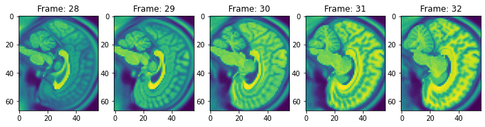
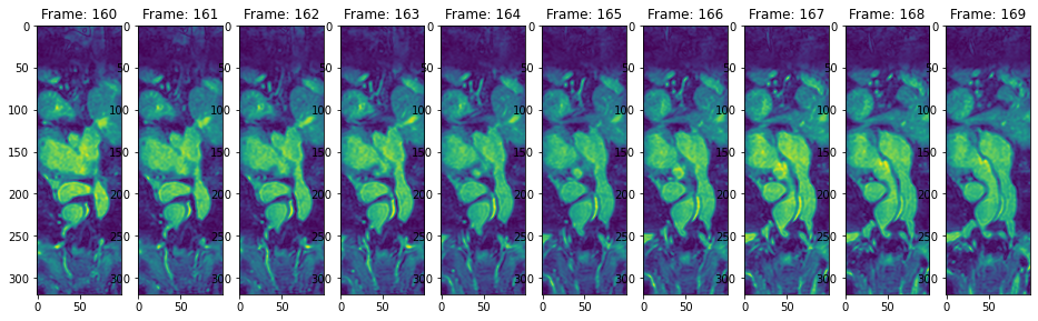
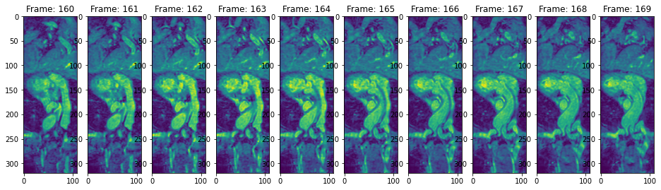
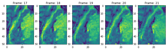
Brain

We shall view the image frames in 2 ways,

1. Pick the frame from the middle and render few subsequent frames
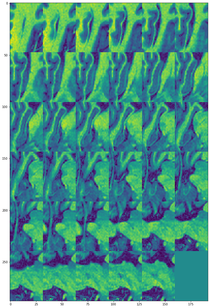
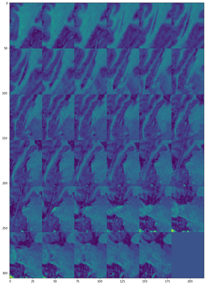
2. View all the frames in 1 plot using montage library

        
view_n_frames(5, data["brain"][0], (12, 12))
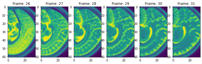
view_n_frames(6, data["brain"][1], (12, 12))

    
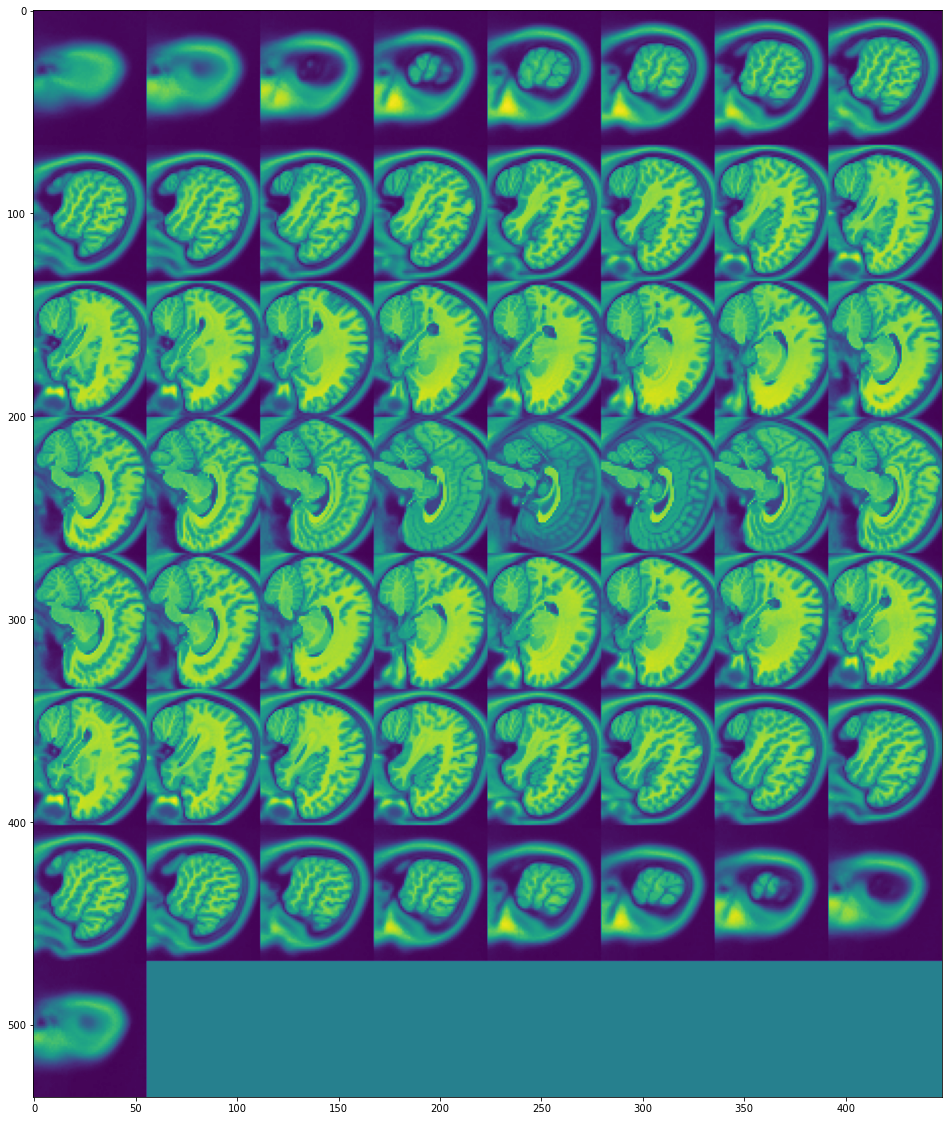
view_all_frames(data["brain"][0], (20, 20))
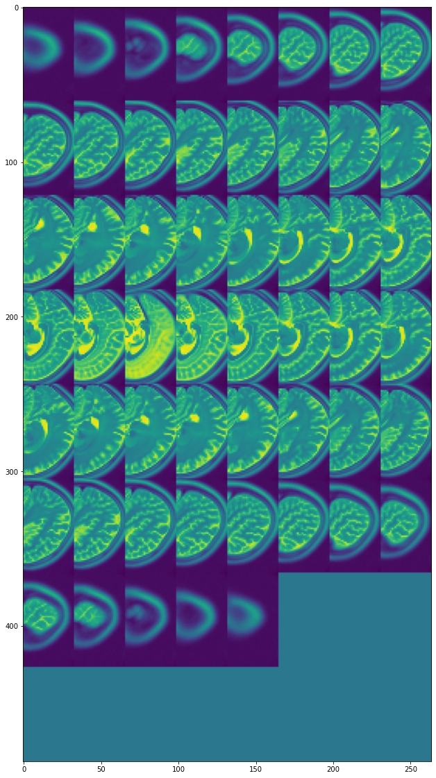
view_all_frames(data["brain"][1], (20, 20))

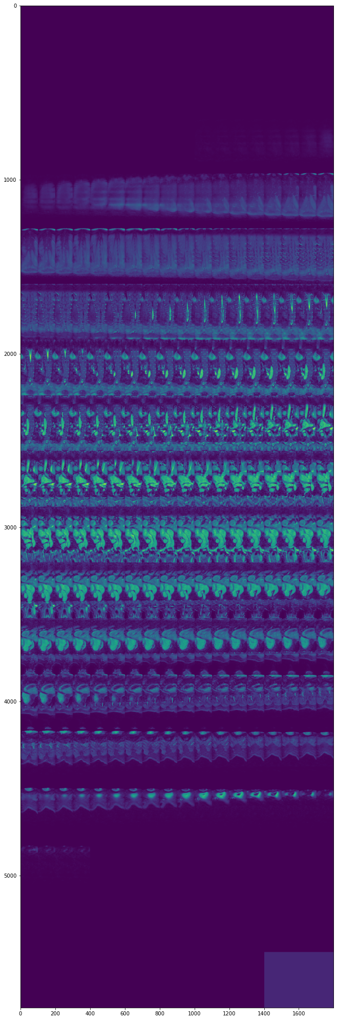
Heart

view_n_frames(10, data["heart"][0], (16, 24))
view_n_frames(10, data["heart"][1], (16, 24))

view_all_frames(data["heart"][0], (12, 36))

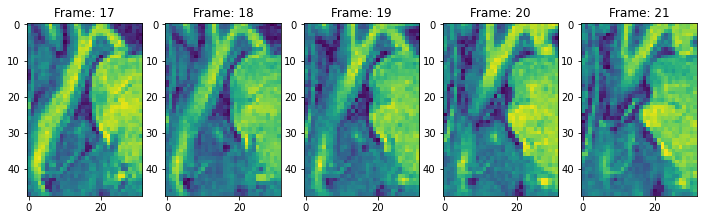
Hippocampus

view_n_frames(5, data["hippocampus"][0], (12, 12))
view_n_frames(5, data["hippocampus"][1], (12, 12))

view_all_frames(data["hippocampus"][0], (12, 24))
view_all_frames(data["hippocampus"][1], (12, 24))

Inference

Our goal was to understand the image construction mechanism of functional magnetic resonance imaging through magnetization principles. We also build a small module that read and visualize open datasets of medical images in NifTI-1 format. This is a significant progress from a spiking neuron modeling to building foundation on fMRIs. This post prepares us to explore the deeper topics like BOLD, k-space etc to enrich our knowledge on neuroscience.

Reference

• Fundamental Physics of MR Imaging by Robert A. Pooley, RadioGraphics
• Detection of COVID-19 from CT scan images: A spiking neural network-based approach
• Principles of fMRI 1 a course by Martin Lindquist, Johns Hopkins University
• Magnetic resonance imaging
• Medical Segmentation Decathlon
• A large annotated medical image dataset for the development and evaluation of segmentation algorithms by Simpson et al
• Image Repo of Medical Segmentation Decathlon