In this post, we shall study the fundamentals of numerical methods by solving Ordinary Differential Equations(ODEs) using our most popular tools includes SciPy, Tensorflow etc. We have solved ODEs and Partial Differential Equations(PDEs) in the past on various occasions in a very simple setup and this post focuses on presenting a practical guide to solve these equations with a mathematical intuition.

Please refer the past posts where we have solved ODEs and PDEs for various purposes here,

• Calculus - Gradient Descent Optimization through Jacobian Matrix for a Gaussian Distribution
• Automatic Differentiation Using Gradient Tapes
• With 20 Watts, We Built Cultures and Civilizations - Story of a Spiking Neuron
• Understanding Post-Synaptic Depression through Tsodyks-Markram Model by Solving Ordinary Differential Equation

I thank Ettore Messina and admire his writings on Math, AI, Quantum Computing under the title Computational Mindset, thought provoking ones. Precious and one of a kind work but less appreciated - Without his scholarly work, this blog post from me wouldn’t have been possible. Also I wish I have learnt Italian, just to comprehend Prof. Fausto D’Acunzo’s lectures at Preparazione 2.0 - What a sweet sounding language Italian is.

Objectives

In this blog post, we shall pick up a simple differential equation and solve them using SciPy and Tensorflow, In that process we shall learn the following

• Cauchy Condition or Initial Value Problem
• Ordinary differential equations
• Numerical analysis and methods to solve ODEs
• Analytical solution for Differential Equation from Wolfram Alpha
• ODE Solvers of TF Probability and SciPy

Introduction

Issac Newton first wrote about Differential Equations in the year 1671 in his book titled Methodus Fluxionum et Serierum Infinitarum, since then the life of most of the students of mathematics become allegedly difficult. Calculus, common cause for excruciating pain and agony among most of the student folks started with 3 differential equations $$\frac{dy}{dx} = f(x)$$ $$\frac{dy}{dx} = f(x, y)$$ $$and$$ $$x_1 \frac{dy}{dx} + x_2 \frac{dy}{dx} = y$$ Where, $y$ is an unknown function$f$ of $x(x_1, x_2)$

The broad classification of differential equations are

1. Partial and Ordinary Differential Equations
2. Linear and Non-Linear Differential Equations and
3. Homogenous and Heterogenous Differential Equations

This list is far from exhaustive; there are many other properties and subclasses of differential equations 
which can be very useful in specific contexts.

- Wikipedia

Numerical Methods

Numerical methods are used for solving functions approximately, we do approximations because of two reasons

1. When the functions cannot be solved exactly and
2. When the functions are intractable to solve exactly, i.e. It takes quite a huge number of simultaneous equations with equally huge number of unknowns

Numerical methods are used to solve various problems and the following are the few to mention

• Find derivatives of continuous and discrete functions
• Solve nonlinear and simultaneous linear equations
• Curve fit discrete data using interpolation and regression
• Find integrals of functions and
• Solve ordinary differential equations(ODE)

ODEs

An ordinary differential equation is an equation defined for one or more functions of ONE independent variable and its derivatives(as opposed to partial derivatives with multiple variables - multivariate). To solve an ODE, our goal is to determine a function or functions that satisfy the equation. If we know the derivative of a function, we can find the function by finding the antiderivative(integrate). Let us see a simple example,

Simplest ODE

$$\frac {dy}{dx} = 0$$ $$then$$ $$f(x) = C$$ In this case, $C$ is a constant and we have no further information to figure out what $C$ is. In such scenarios, we seek more data to approximate the value of $C$. For example, $C=24$ when $x=8$, $C=21$ when $x=7$ and so on and so forth. The idea of knowing $C=24$ when $x=8$ is intial condition.

Cauchy’s Condition

It has too many names and I think it is just to credit too many individuals who had come up with the idea. Few names that I bumped into are

1. Initial Value Problem
2. Cauchy’s Condition - btw who is Cauchy? Augustin-Louis Cauchy and
3. Cauchy Boundary Condition

It just denotes, we have to start from somewhere and let us set some initial values to place the problem within a boundary. Like the one we have defined for our Simple ODE function.

Let Us Complicate Things

It is fun to have time $t$ into our analysis, consider an equation $$\frac {dx}{dt} = - c_1 cos(t) + c_2 t^2$$ Where, $(c_1, c_2)$ are some constants or real numbers and we have specified the derivative in time domain.

Let us, take the integral between a time period $a, b$ - i.e. definite integral at $t: a \rightarrow b$. $$x(b) - x(a) = \int_a^b \frac {dx}{dt} dt$$ $$x(b) - x(a) = \int_a^b (- c_1 cos(t) + c_2 t^2) dt$$ $$x(b) - x(a) = - c_1 sin(b) + c_2 \frac{b^3}{3} - ( - c_1 sin(a) + c_2 \frac{a^3}{3})$$ $$or$$ $$x(t) = - c_1 sin(t) + c_2 \frac{t^3}{3} + C$$ Where, $C$ is an arbitrary constant.

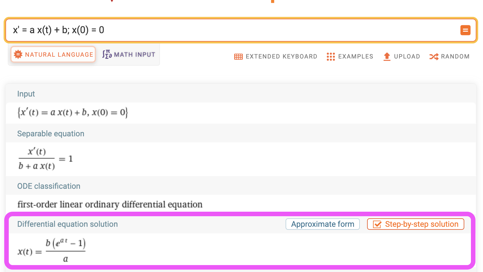
BTW, things are not always as simple as the above examples, Let us take the following example $$\frac {dx}{dt} = c_1 x(t) + c_2$$ $$\text{RHS has both x and t, makes things more interesting but beyond the scope of this post}$$ Solving for $x(t)$ result in, $$x(t) = \frac{1}{a}log |ax(t) + b| + C$$

Let us set our initial condition $x(t) = 0$ and find the function of our interest $$\frac{1}{a}log |ax(t) + b| + C = 0$$

We shall use WolframAlpha to figure out the function for the initial condition $x(0) = 0$,

Solving ODEs

This section is totally inspired by Ettore Messina’s blog posts, I learnt a lot from his articles and tried to mock the same with my own style. The objective of this section is to pick a simple differential equation and solve it using

1. SciPy and
2. TF Probability

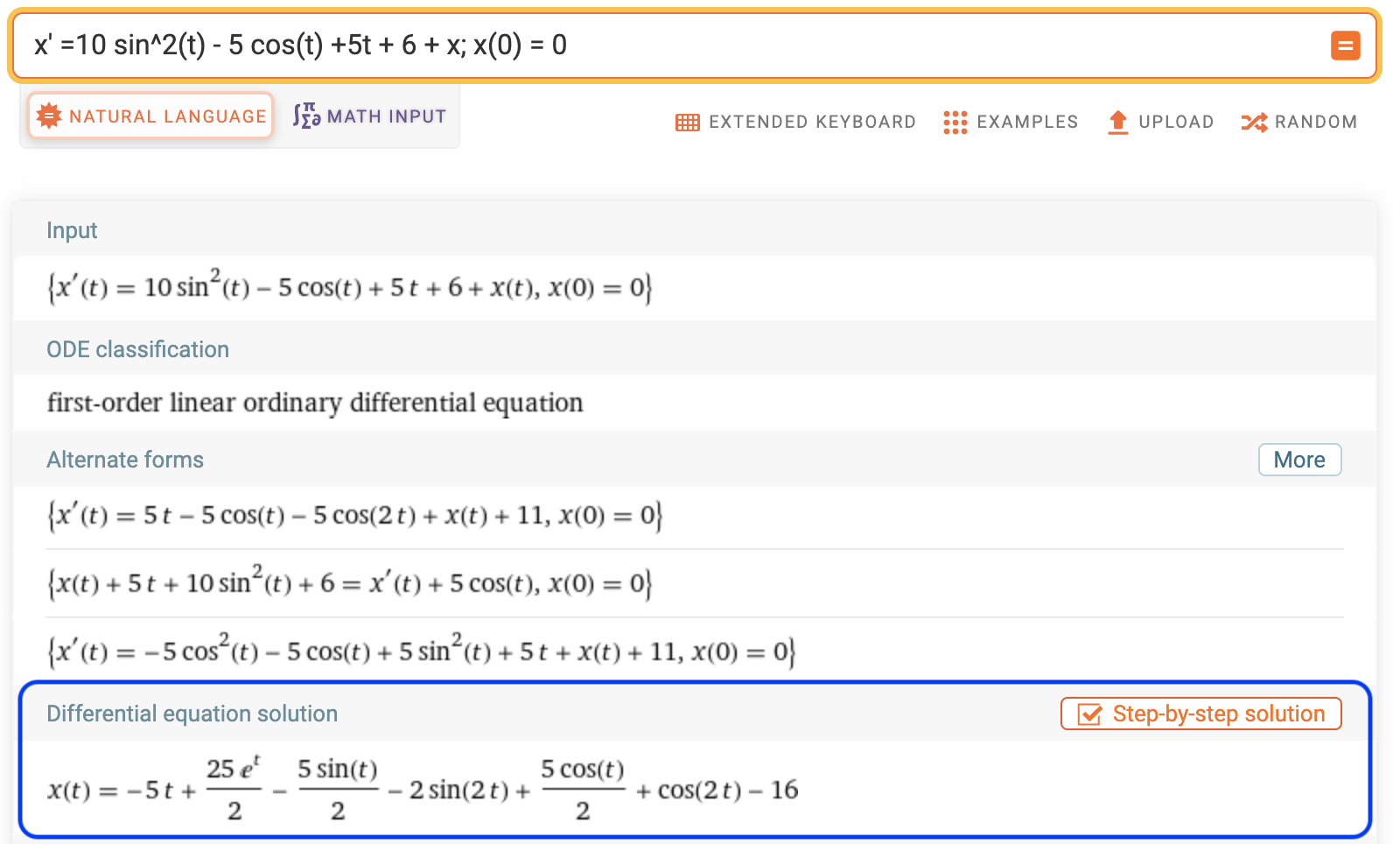
Our differential equation under the hammer is a similar one that we studied in the previous section with some modifications. $$\frac {dx}{dt} = 10 sin^2(t) - 5 cos(t) +5t + 6 + x \tag{1}$$ $$\text{Initial Condition, }x(0) = 0$$ $$then$$ $$x(t) = -5t + \frac{25e^t}{2} - \frac {5sint(t)}{2} - 2sin(2t) + \frac{5cos(t)}{2} + cos(2t) - 16 \tag{2}$$

We shall use WolframAlpha to figure out the function for the initial condition $x(0) = 0$,

import numpy as np
import math
dx_dt = lambda t, x: (10 * (np.sin(t) **2))  - (5 * np.cos(t) )+ (5 * t) + 6 + x
f_x = lambda t: -5*t + 25 * np.exp(t) / 2 - 5 * np.sin(t)/2 - 2 * np.sin(2*t) + 5 * np.cos(t) / 2 + np.cos(2*t) - 16
t_BEGIN = 0
t_END = 10
n_SAMPLES = 100
t_SPACE = np.linspace(t_BEGIN, t_END, n_SAMPLES)
x_INIT = 0.

x_ANALYTICAL = f_x(t_SPACE)

import matplotlib.pyplot as plt

def plot_util(method, space,  analytical, times, numerical):
    fig, axs = plt.subplots(1, 2, figsize=(15, 5))
    fig.suptitle(f"Solving 1st Order ODE - {method}", size=24)

    axs[0].plot(space, analytical, linewidth=2)
    axs[0].set_title('Analytical')
    axs[0].set_xlabel('t')
    axs[0].set_ylabel('x')
    axs[1].plot(times, numerical, linewidth=2, color="green")
    axs[1].set_title('Numerical')
    axs[1].set_xlabel('t')
    axs[1].set_ylabel('x')
    plt.show()

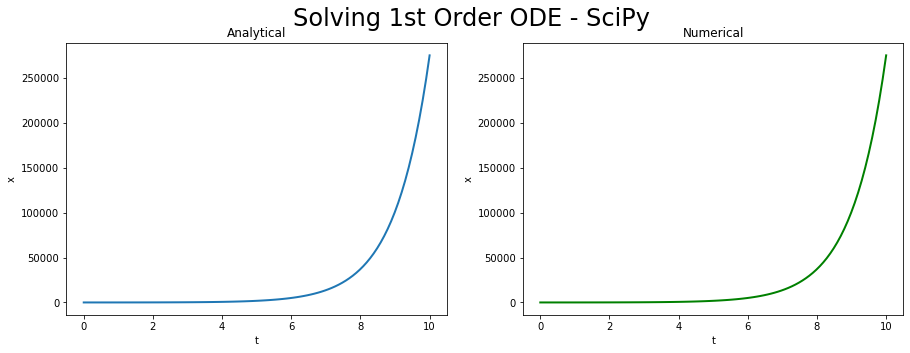
SciPy

from scipy.integrate import solve_ivp
num_sol = solve_ivp(dx_dt, [t_BEGIN, t_END], [x_INIT], method='RK45', dense_output=True)
x_NUMERICAL = num_sol.sol(t_SPACE).T
plot_util("SciPy", t_SPACE, x_ANALYTICAL, t_SPACE, x_NUMERICAL)

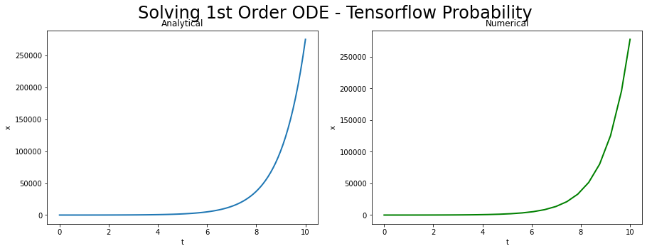
TF Probability

import tensorflow as tf
import tensorflow_probability as tfp
dx_dt = lambda t, x: (tf.constant(10.) * (tf.math.sin(t) **2))  - (tf.constant(5.) * tf.math.cos(t) )+ (tf.constant(5.) * t) + tf.constant(6.) + x

x_NUMERICAL = tfp.math.ode.BDF().solve(
    dx_dt,
    tf.constant(t_BEGIN),
    tf.constant(x_INIT),
    solution_times=tfp.math.ode.ChosenBySolver(tf.constant(t_END))
)

WARNING:tensorflow:5 out of the last 5 calls to <function pfor.<locals>.f at 0x7fd3382ca160> triggered tf.function retracing. Tracing is expensive and the excessive number of tracings could be due to (1) creating @tf.function repeatedly in a loop, (2) passing tensors with different shapes, (3) passing Python objects instead of tensors. For (1), please define your @tf.function outside of the loop. For (2), @tf.function has experimental_relax_shapes=True option that relaxes argument shapes that can avoid unnecessary retracing. For (3), please refer to https://www.tensorflow.org/guide/function#controlling_retracing and https://www.tensorflow.org/api_docs/python/tf/function for  more details.
WARNING:tensorflow:6 out of the last 6 calls to <function pfor.<locals>.f at 0x7fd331bce790> triggered tf.function retracing. Tracing is expensive and the excessive number of tracings could be due to (1) creating @tf.function repeatedly in a loop, (2) passing tensors with different shapes, (3) passing Python objects instead of tensors. For (1), please define your @tf.function outside of the loop. For (2), @tf.function has experimental_relax_shapes=True option that relaxes argument shapes that can avoid unnecessary retracing. For (3), please refer to https://www.tensorflow.org/guide/function#controlling_retracing and https://www.tensorflow.org/api_docs/python/tf/function for  more details.

plot_util('Tensorflow Probability', t_SPACE, x_ANALYTICAL, x_NUMERICAL.times, x_NUMERICAL.states)

Conclusion

I am so grateful that I got the opportunity to read Ettore Messina’s blog posts, It made a big impact on me and once again remind me there is so much to learn. This post is nothing but a mock of one of his posts where I had the opportunity to learn ODEs. In this post, we derived a simplistic form of ODE and built a sophisticated one and moved up high with a complex ODE function. Subsequently in the second section, we solved a first order ODE using SciPy and Tensorflow Probability. I strongly recommend Messina’s blog for solving 2 ODEs of first order with IVP, Its fun.

References

• Ordinary differential equation solvers in Python by Ettore Messina
• Computational Mindset - SCIENCE & TECHNOLOGY WEBSITE Personal Portfolio of Ettore Messina
• Welcome to the world of approximations - Numerical Methods by Prof. Autar Kaw, USF
• An introduction to ordinary differential equations from Math Insight
• Initial Value Problem from Wikipedia
• Differential Equations from Wikipedia
• Methods of Fluxions from Wikipedia about Newton’s Methodus Fluxionum et Serierum Infinitarum
• First and Second Order ODEs by M.Ottobre, 2011
• Wolfram Alpha, Solve: x’ =10 sin^2(t) - 5 cos(t) +5t + 6 + x; x(0) = 0