Furthermore, we measure the decision tree accuracy using confusion matrix with various improvement schemes.

[25th Apr 2021, Note to the reader]: Gini index in the title of the post is misleading and I have some challenges in fixing it. We are discussing Gini Impurity, Gini Index has no relevance to this post.

Previous Posts in this Series

• Bayesian and Frequentist Approach to Machine Learning Models
• Understaning Uncertainty, Deterministic to Probabilistic Neural Networks
• Shannon’s Entropy, Measure of Uncertainty When Elections are Around
• KL-Divergence, Relative Entropy in Deep Learning

I recommend Classification Trees in Python, From Start To Finish short course by Josh Starmer. Without his course, this article wouldn’t have reached this finishing stage.

Image Credit: Portland Japanese Garden – Living in Harmony with Nature

Objective

Our primary goal is to conclude this series of articles by taking a real dataset and measure uncertainty under a controlled setup. With that quest in mind, this post should answer the following questions

• What is Information Gain?
• What is Gini Impurity?
• Recap of Entropy and KL Divergence
• How KL divergence and Entropy is related to Information Gain?
• Is Mutual Information and Information Gain are same?
• What is a Decision Tree
• Decision making using Decision Trees
• How information gain helps to optimize the trees?
• How to calculate information gain?
• Compare IG of a manual split and optimized split
• Introduce Cost Complexity Pruning

Introduction

Information gain calculates the reduction in entropy or uncertainty by transforming the dataset towards optimum convergence. It compares the dataset before and after every transformation to arrive at reduced entropy.
From our previous post, we know entropy is $$H(X) = - \sum_{i=1}^n p_i log_2 p_i \tag{1. Entropy}$$

KL-Divergence - It is the amount of information gained about a random variable from observing another random variable. In our KL-Divergence post, we coined it as difference of two distributions rather than two random variables. Due to this simple reason, KL-Divergence and Information gain are synonymous. However, In the context of random variable, we call it Mutual Information.

$$\mathbb{E_p}\left[log \frac {p_{\theta}(x)}{q_{\phi}(x)}\right ] = \sum_{i=1}^{\infty}p_{\theta}(x_i)\left[log \frac {p_{\theta}(x_i)}{q_{\phi}(x_i)}\right ] \tag{2. KL-Divergence}$$

Information Gain (Mutual Information)

Let $(X, Y)$ be a pair of random variables in their space, If their joint distribution is $P_{(X, Y)}$ and the marginal distributions are $P_X$ and $P_Y$ then $$I(X;Y) = D_{KL}(P_{(X, Y)} || P_X \otimes P_Y) \tag{3a}$$

The above equation is bit difficult to comprehend but it is all talking about prior distribution, posterior distribution etc of KL-Divergence. Let us rewrite the same equation as follows
$$IG_{X, Y}(X, y) = D_{KL}(P_X(x|y) || P_X(x|I)) \tag{3b}$$ i.e. The information gain of a random variable $X$ from an observation A for a value A = a. Where,

• $P_X(x|I)$ is the prior distribution
• $P_{X|Y}(x|y)$ is posterior distribution for x given y

Note: The reduction in the entropy of X is achieved by learning the state of the random variable $Y$

$eqn.3a/b$ can be written as
$$I(X;Y) = \sum_{x \in X, y \in Y} p_{(X, Y)}(x, y) log \frac {p_{(X, Y)}(x, y)}{p_X(x)p_Y(y)}$$ $$i.e.$$ $$\sum_{x \in X, y \in Y} p_{(X, Y)}(x, y) log \frac {p_{(X, Y)}(x, y)}{p_X(x)} - \sum_{x \in X, y \in Y} p_{(X, Y)}(x, y) log p_Y(y)$$

let us split the equations by decluttering the joint probability factors

$$\sum_{x \in X, y \in Y} p_X(x)p_{Y|X=x}(y) log p_{Y|X=x}(y) - \sum_{x \in X, y \in Y} p_{(X, Y)}(x, y) log p_Y(y)$$

$$\sum_{x \in X}p_X(x)\left(\sum_{y \in Y} p_{Y|X=x}(y) log p_{Y|X=x}(y) \right) - \sum_{y \in Y} \left ( \sum_{x \in X} p_{(X, Y)}(x, y) \right) log p_Y(y)$$

There are 2 terms inside the big brackets…

• $\sum_{y \in Y} p_{Y|X=x}(y) log p_{Y|X=x}(y) \rightarrow -H(Y|X)$ the conditional entropy of a joint distribution
• $\sum_{x \in X} p_{(X, Y)}(x, y) \rightarrow p_Y(y)$ ie the probability of $y$ for all $x$

This equation looks a lot familiar now. $$\sum_{x \in X}p(x)H(Y|X=x) - \sum_{y in Y}p_Y logp_Y(y)$$ $i.e$ $$I(X;Y) = -H(Y|X) + H(X)$$ $$I(X;Y) = H(Y) - H(Y|X) \tag{4. Information Gain}$$

Decision Trees

In decision trees, we have to make an optimal split at the root node and subsequent nodes for quick convergence. To achieve this classification trees use Gini Impurity and Information Gain.

Gini Impurity

Gini Impurity tells, what is the probability that an item is mis-classified. It can be computed by summing the probability $p_i$ of an item with label i being chosen times the probability $1 - p_i$ of mistake in categorizing them. Let us say, we have N different classes in our sample set then

$$Gini_{impurity} = p_1.(1-p_1) + p_2.(1-p_2) + p_3.(1-p_3) + \cdots + p_N.(1-p_N)$$ $$i.e.$$ $$Gini_{impurity} = 1 - \sum_{i=1}^N p_i^2$$

Information Gain in Decision Trees

Let $T$ denotes a set of $N$ observations of a dataset $(x, y) = (x_1, x_2, x_3, \dots, x_N, y)$ with their labels $y$ - $y$ can be discrete or continous. Then information gain for a parameter $a$ is defined in terms of Shannon's Entropy $H(T)$ i.e. $$IG(T,a) = H(T) - H(T|a)$$

• $H(T|a)$ is the conditional entropy

$$H(T|a) = \mathbb{E}_{P_a} [H(S_a(v))] = \sum \frac{|S_a(v)|}{|T|}. H(S_a(v)) \tag{5. Expectation Value}$$

For a value $v$ taken from a parameter $a$, let $$S_a(v) = {x \in T | x_a = v}$$

From a decision tree point of view,

$$\Large \overbrace{IG(T,a)}^{Information\ Gain} = \underbrace{H(T)}_{Entropy\ of\ Parent} - \overbrace{H(T|a)}^{Sum\ of\ Entropies\ of\ Children}$$

Calculating Information Gain using UCI Heart Disease Dataset

In this section we shall see how to calculate information gain using UCI Heart Disease Dataset and compare an unoptimized tree with optimized tree.

• Acquire the data from UCI Repository
• Split the data into train and test set
• Create a random split manually
• Calculate the Information Gain for the random split
• Introduce pruning
• Fit the train data using DecisionTreeClassifier of Sklearn with optimum alpha value
• Plot the tree using the fitted model
• Calculate the information gain of the plotted tree
• Compare the information gain of optimized tree from the classifier and the random tree manually created

from trees import get_data
import pandas as pd # load and manipulate data and for One-Hot Encoding
import numpy as np # calculate the mean and standard deviation
import matplotlib.pyplot as plt # drawing graphs
from sklearn.tree import DecisionTreeClassifier # a classification tree
from sklearn.tree import plot_tree # draw a classification tree
from sklearn.model_selection import train_test_split # split  data into training and testing sets
from sklearn.model_selection import cross_val_score # cross validation
from sklearn.metrics import confusion_matrix # creates a confusion matrix
from sklearn.metrics import plot_confusion_matrix # draws a confusion matrix

def entropy(splits):
    """
    Entropy
    Entropy is the measure of uncertainty between two variables
    """
    total = splits[0] + splits[1]
    return - (splits[0] / total) * np.log2(splits[0] / total) - (splits[1] / total) * np.log2(splits[1] / total)

def info_gain(current_uncertainty, total, left, right):
    """
    Information Gain.

    The uncertainty of the starting node, minus the weighted impurity of
    two child nodes.
    """
    p1 = sum(left) / total
    p2 = sum(right) / total
    uncertainty_left = entropy(left)
    uncertainty_right = entropy(right)
    
    return current_uncertainty - (p1 * uncertainty_left + p2 * uncertainty_right)

Manual Split by Randomly Picking Features

Our goal is to create a tree as follows. I did an exploratory analysis on the data set and picked two features

1. oldpeak, our first split is $oldpeak >= 2.7$
2. age, our second split is $age >= 55$

For simplicity, I moved all the preprocessing code to a python utility get_data method does all the magics

X_train, X_test, y_train, y_test = get_data()
oldpeak_left = X_train[X_train["oldpeak"] <= 2.7]
oldpeak_right = X_train[X_train["oldpeak"] > 2.7]
print(f'Old Peak Left Count: {len(oldpeak_left)}, Right Count: {len(oldpeak_right)}')

age_left_left = oldpeak_left[oldpeak_left["age"] <= 55]
age_left_right = oldpeak_left[oldpeak_left["age"] > 55]
print(f'Old Peak Left - Age Left Count: {len(age_left_left)}, Age Right Count: {len(age_left_right)}')

age_right_left = oldpeak_right[oldpeak_right["age"] <= 55]
age_right_right = oldpeak_right[oldpeak_right["age"] > 55]
print(f'Old Peak Right - Age Left Count: {len(age_right_left)}, Age Right Count: {len(age_right_right)}')

Old Peak Left Count: 200, Right Count: 22
Old Peak Left - Age Left Count: 103, Age Right Count: 97
Old Peak Right - Age Left Count: 9, Age Right Count: 13

parent_split = [200, 22]
child_split_left = [103, 97]
child_split_right = [9, 13]
H_T = entropy(parent_split)

gain_manual_split = info_gain(H_T, sum(parent_split), child_split_left, child_split_right)
gain_manual_split

-0.5309054209881511

Cost Complexity Pruning

Decision trees generally overfit to the training dataset, pruning is done to improve the accuracy on test dataset. The pruning process involves identifying the right pruning parameter $\alpha_{cc}$ . Cost complexity pruning is beyond the scope of this article.

def create_dt_classifier(X_train, y_train, ccp_alpha=0.0):
    classifier = DecisionTreeClassifier(
        random_state=42, 
        ccp_alpha=ccp_alpha
    )
    classifier.fit(X_train, y_train)
    
    plot_tree(
        classifier, 
        filled=True, 
        rounded=True, 
        class_names=["No HD", "Yes HD"], 
        feature_names=X_train.columns
    )
    
    return classifier

Let us build a DecisionTreeClassifier with $\alpha_{cc} = 0.09$ and train the network. Subsequently, we shall render the classification tree as well.

import matplotlib.pyplot as plt
plt.figure(figsize=(10,5))
classifier = create_dt_classifier(X_train, y_train, ccp_alpha=0.09)

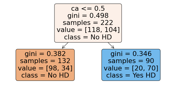
This optimized tree picks the right splits by starting with ca values. Let us see the efficacy of this tree on the test dataset as well by rendering the confusion matrix.

parent_split = [118, 104]
child_split_left = [98, 34]
child_split_right = [20, 70]
H_T = entropy(parent_split)

gain_optimized_tree = info_gain(H_T, sum(parent_split), child_split_left, child_split_right)
print(f"Information Gain for CC_Alpha = 0.09 is {gain_optimized_tree}") 

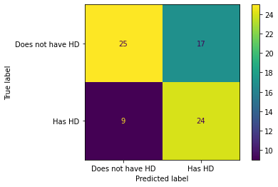
plot_confusion_matrix(classifier, X_test, y_test, display_labels=["Does not have HD", "Has HD"])

Information Gain for CC_Alpha = 0.09 is 0.19792605316695





<sklearn.metrics._plot.confusion_matrix.ConfusionMatrixDisplay at 0x7f9784d7b130>

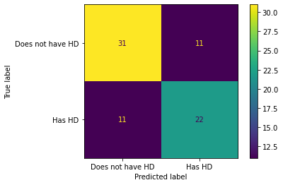
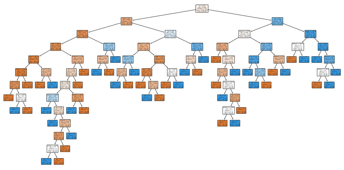
Optimized Tree with $\alpha=0.01422$

Using cost complexity pruning methodology, a right alpha is identified as 0.01422, using this value we shall build a new classifier and

plt.figure(figsize=(15,10))
classifier = create_dt_classifier(X_train, y_train, ccp_alpha=0.014224751066856332)

plot_confusion_matrix(classifier, X_test, y_test, display_labels=["Does not have HD", "Has HD"])

<sklearn.metrics._plot.confusion_matrix.ConfusionMatrixDisplay at 0x7f9784d49910>

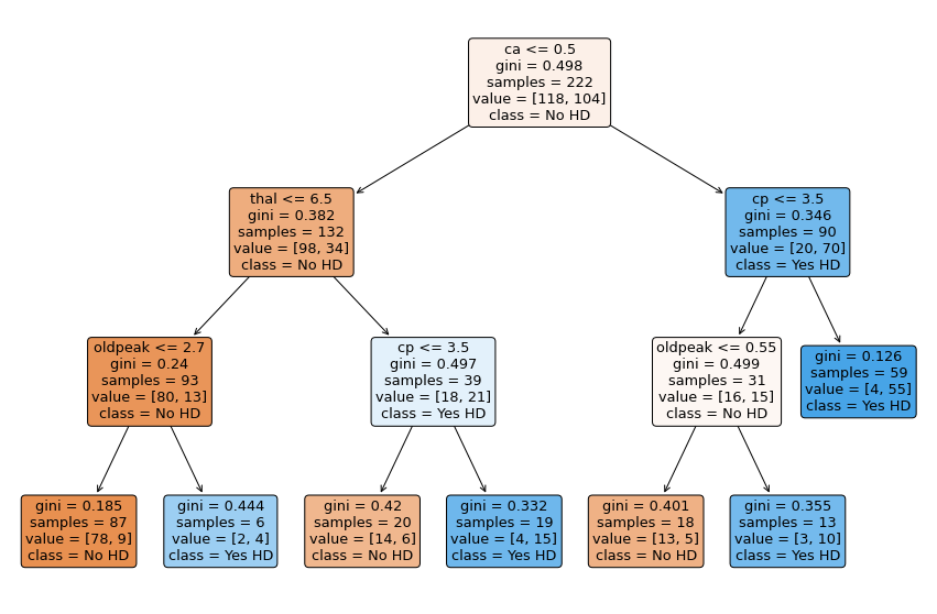
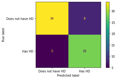
Without Pruning

The effect of cost complexity pruning is significant, on the same UCI Heart Disease dataset - Decision Tree Classifier overfit the tree. The inefficiency of the tree can be observed below with the plot and confusion matrix.

plt.figure(figsize=(20,10))
classifier = create_dt_classifier(X_train, y_train)
plot_confusion_matrix(classifier, X_test, y_test, display_labels=["Does not have HD", "Has HD"])

<sklearn.metrics._plot.confusion_matrix.ConfusionMatrixDisplay at 0x7f9784fa1370>

Inference

I believe we are able to answer all the questions we wanted answers in the objective section. Further we built couple of classifiers on the Heart Disease dataset

• Our Information Gain on manual split is quite lower than the optimized split
• From the confusion matrix,
  • An unoptimized classifier accuracy was 65.33%
  • With random $\alpha_{cc} = 0.09$ accuracy was 70.66%
  • With optimized $\alpha_{cc} = 0.014$ accuracy was 82.66%

Reference

• Mutual information
• Information gain in decision trees
• Gini Impurity
• Gini Impurity Measure – a simple explanation using python
• Tutorial 38- Decision Tree Information Gain
• Information Gain in KL-D
• Decision Trees in Python from Start to Finish