Graph Convolution Network - A Practical Implementation of Vertex Classifier and it's Mathematical Basis
Posted September 25, 2021 by Gowri Shankar ‐ 10 min read
Traditional deep learning algorithms work in the Euclidean space because the dataset is transformed and represented in one or two dimensions. This approach results in loss of information, especially on the relationship between two entities. For example, the network organization of the brain suggests that the information is stored in the neuronal nexus. i.e Neurons fire together, wire together - Hebbian Theory. The knowledge of togetherness or relationships can be ascertained strongly in the non-Euclidean space in the form of Graphs Networks. Such intricate graph networks are evolved to maximize efficiency and efficacy in the form of information transfer at a minimum cost(energy utilization) to accomplish complex tasks. Though the graph networks solve the spatial challenges to certain extents, temporal challenges are yet to be addressed. Extending DNN theories with the graph is the current trend, e.g. an image can be considered as a specialized graph where the pixels have relation to their adjacent ones, to perform a Graph Convolution.
In this post, we shall realize a Graph Convolution Network(GCN) inspired by a few popular pieces of literary work and study the mathematical foundation behind it. This is our second post on Graphs and Graph Neural Networks where I tried my best to render the ideas from theory to practical implementation. Please refer to the previous post here,

- Image Credit: A Comprehensive Survey on Graph Neural Networks
This post is a walk-through of Khalid Salama’s tutorial on Node Classification with Graph Neural Networks. I thank Khalid for his simplified explanation of GCN and its implementation.
Objective
The primary objective of this post is to implement the GCN concept using Tensorflow and our goal is to implement the Graph Convolution Layer from scratch. In this quest, We shall study the math behind GCNs.
Introduction
We are building a Graph Convolution based Graph Neural Network in this post, our data comes from the Cora dataset consists of scientific publications classified into one of 7 classes. Total 2708 scientific papers are classified as follows,
- Neural_Networks (818)
- Probabilistic_Methods (426)
- Genetic_Algorithms (418)
- Theory (351)
- Case_Based (298)
- Reinforcement_Learning (217)
- Rule_Learning (180)
The Cora dataset consists of 2708 scientific publications classified
into one of seven classes. The citation network consists of 5429 links.
Each publication in the dataset is described by a 0/1-valued word vector
indicating the absence/presence of the corresponding word from the
dictionary. The dictionary consists of 1433 unique words.

- Cora by Arnaud Barragao
Our focus is more towards understanding the GNN architecture and the math behind it rather than arriving at a perfect graph model that classifies the publications based on the citations. Further, this post covers ideas present in the following 4 papers
- Gated Graph Sequence Neural Networks
- Simplifying Graph Convolutional Networks
- How Powerful Are Graph Neural Networks
- Inductive Representation Learning on Large Graphs
- Semi-Supervised Classification With Graph Convolution Networks
import tensorflow as tf
import matplotlib.pyplot as plt
from utils import read_data, preprocess, visualize_graph, train_test_split, train_fn, display_learning_curves, create_ffn
Dataset and Preprocessing
I have written a few utility functions to download the data from the Cora repository and preprocess it. subject column points to the class of the publications and the columns with the prefix term is the presence of a term marked ${0, 1}$ for absence and presence respectively. The term columns are our feature vector for the publication identified by the paper_id column.
In our second table, we have the citation record with two columns, target where the cited paper id is mentioned and source the paper of interest. We convert the paper_ids and subject to the zero-based index for easy processing.
papers, citations = read_data()
papers_orig = papers.copy()
citations_orig = citations.copy()
print(papers.shape, citations.shape)
(2708, 1435) (5429, 2)
papers.head()
| paper_id | term_0 | term_1 | term_2 | term_3 | term_4 | term_5 | term_6 | term_7 | term_8 | ... | term_1424 | term_1425 | term_1426 | term_1427 | term_1428 | term_1429 | term_1430 | term_1431 | term_1432 | subject | |
|---|---|---|---|---|---|---|---|---|---|---|---|---|---|---|---|---|---|---|---|---|---|
| 0 | 31336 | 0 | 0 | 0 | 0 | 0 | 0 | 0 | 0 | 0 | ... | 0 | 0 | 1 | 0 | 0 | 0 | 0 | 0 | 0 | Neural_Networks |
| 1 | 1061127 | 0 | 0 | 0 | 0 | 0 | 0 | 0 | 0 | 0 | ... | 0 | 1 | 0 | 0 | 0 | 0 | 0 | 0 | 0 | Rule_Learning |
| 2 | 1106406 | 0 | 0 | 0 | 0 | 0 | 0 | 0 | 0 | 0 | ... | 0 | 0 | 0 | 0 | 0 | 0 | 0 | 0 | 0 | Reinforcement_Learning |
| 3 | 13195 | 0 | 0 | 0 | 0 | 0 | 0 | 0 | 0 | 0 | ... | 0 | 0 | 0 | 0 | 0 | 0 | 0 | 0 | 0 | Reinforcement_Learning |
| 4 | 37879 | 0 | 0 | 0 | 0 | 0 | 0 | 0 | 0 | 0 | ... | 0 | 0 | 0 | 0 | 0 | 0 | 0 | 0 | 0 | Probabilistic_Methods |
5 rows × 1435 columns
citations.head()
| target | source | |
|---|---|---|
| 0 | 35 | 1033 |
| 1 | 35 | 103482 |
| 2 | 35 | 103515 |
| 3 | 35 | 1050679 |
| 4 | 35 | 1103960 |
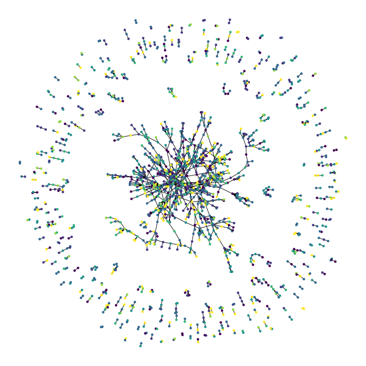
papers, citations, class_values, class_idx, paper_idx = preprocess(papers, citations)
visualize_graph(papers, citations)
Features, Train/Test Splitting
The method train_test_split randomly samples half the data for training and the remaining half for testing.
train_data, test_data = train_test_split(papers)
feature_names = set(papers.columns) - {"paper_id", "subject"}
num_features = len(feature_names)
num_classes = len(class_idx)

x_train = train_data[feature_names].to_numpy()
x_test = test_data[feature_names].to_numpy()
y_train = train_data["subject"]
y_test = test_data["subject"]
Train data shape: (1337, 1435)
Test data shape: (1371, 1435)
Graph Data Preparation
Preparing data for a graph model is the most cumbersome part of the GNN models. We are taking a simple approach by constructing the following
- Node Features: This is the feature matrix that represents the
termspresent in the literature of dimension ${n_{nodes} \times n_{features}}$ - Edges: An adjacency matrix represented as a sparse matrix of dimension ${n_{edge} \times n_{edge}}$
- Edge Weight: We consider all edges are equally weighted and it is $1^s$ of feature count.
edges = citations[["source", "target"]].to_numpy().T
edge_weights = tf.ones(shape=edges.shape[1])
node_features = tf.cast(
    papers.sort_values("paper_id")[feature_names].to_numpy(), dtype=tf.dtypes.float32
)
graph_info = (node_features, edges, edge_weights)
print("Edges shape:", edges.shape)
print("Nodes shape:", node_features.shape)
Edges shape: (2, 5429)
Nodes shape: (2708, 1433)
Building a GNN Model
This section has 2 parts,
- Building a Graph Convolution Layer from the scratch in Tensorflow without using any sophisticated graph libraries
- Subsequently build a GNN Node Classifier using a Feed-Forward Network and the Graph Convolution Layer
Following are the hyperparameters used for training the model.
Graph Convolution Layer Basics
Graph convolution module performs 3 steps,
- Linear Transformation
- Neighborhood Aggregation Strategy
- Readout Functions
Before getting into the details, let us bring in the mathematical basis for GNN models
$$let$$ $$\Large G = (V, E) \tag{1. Graph}$$ Where,
- $V$ is the vertex and $E$ is the edges
- Each vertex has its associated node feature$(X_v)$ for $v \in V$, In Cora dataset the
termsare the feature $v$
In general, we have two tasks,
- Node Classification, where each node $v \in V$ has an associated label $y_v$,
subjectin our case. Learn a representation vector $h_v$ of $v$ such that $v$’s labes can be predicted as $$\Large y_v = f(h_v) \tag{2. Node Classification}$$ - Graph Classification(not in the scope of this article), for a set of graphs ${G_1, G_2, G_3, \cdots, G_N} \subseteq \mathcal{G}$ and their labels ${y_1, y_2, y_3, \cdots, y_N} \subseteq \mathcal{Y}$, we aim to learn a representation vector $h_G$ that helps to predict the entire graph as $$\Large y_G = g(h_G)\tag{3. Graph Classification}$$
Linear Transformation
The first step in constructing a GCN layer is to process the input node representation using a Feed-Forward Network to produce a message.
Neighborhood Aggregation Strategy and Readout
GNNs follow an aggregation strategy where we iteratively update the representation of a node by aggregating representations of its neighbors. After $k$ iterations of aggregation, a node’s representation captures the structural information within its k-hop network neighborhood.
$$a_v^{(k)} = AGGREGATE^{(k)}\left({ h_u^{(k-1)}: u \in \mathcal{N}(v)}\right) \tag{4. Aggregate Method GraphConvLayer}$$ $$h_v^{(k)} = COMBINE^{(k)}\left(h_v^{k-1}, a_v^{(k)}\right) \tag{5. Update Method GraphConvLayer}$$
Where,
- $h_v^{(k)}$ is the feature vector of node $v$ at the $k^{th}$ iteration layer.
- $h_v^{(0)}$ is initialized to $X_v$ during the beginning of the iteration
- $\mathcal{N}(v)$ is a set of nodes adjacent to $v$
A number of architectures for AGGREGATE have been proposed
1. Element-wise Max Pooling variant of GraphSAGE (Hamilton et al., 2017a)
2. Element wise Mean Pooling variant of GCN ((Kipf & Welling, 2017)

- Xu et al, How Powerful Are GNN - ICLR 2019

Image Credit: Inductive Representation Learning on Large Graphs
We use modified element-wise mean pooling variant of GCN proposed by Kipf & Welling.
The node representation $h_v^{(K)}$ of the final iteration is used for prediction.
The node_repesentations and aggregated_messages—both of shape [num_nodes, representation_dim]—
are combined and processed to produce the new state of the node representations (node embeddings).
If combination_type is gru, the node_repesentations and aggregated_messages are stacked to create
a sequence, then processed by a GRU layer. Otherwise, the node_repesentations and aggregated_messages
are added or concatenated, then processed using a FFN.

- Khalid Salama
# This code belongs to Khalid Salama
class GraphConvLayer(tf.keras.layers.Layer):
    def __init__(
        self,
        hidden_units,
        dropout_rate=0.2,
        aggregation_type="mean",
        combination_type="concat",
        normalize=False,
        *args,
        **kwargs
    ):
        super(GraphConvLayer, self).__init__(*args, **kwargs)

        self.aggregation_type = aggregation_type
        self.combination_type = combination_type
        self.normalize = normalize

        self.ffn_prepare = create_ffn(hidden_units, dropout_rate)

        if(self.combination_type == "gated"):
            self.update_fn = tf.keras.layers.GRU(
                units=hidden_units,
                activation="tanh",
                recurrent_activation="sigmoid",
                dropout=dropout_rate,
                return_state=True,
                recurrent_dropout=dropout_rate
            )
        else:
            self.update_fn = create_ffn(hidden_units, dropout_rate)

    def prepare(self, node_representations, weights=None):
        messages = self.ffn_prepare(node_representations)
        if(weights is not None):
            messages = messages * tf.expand_dims(weights, -1)
        return messages

    def aggregate(self, node_indices, neighbour_messages):
        num_nodes = tf.math.reduce_max(node_indices) + 1
        if(self.aggregation_type == "sum"):
            aggregated_message = tf.math.unsorted_segment_sum(
                neighbour_messages, node_indices, num_segments=num_nodes
            )
        elif(self.aggregation_type == "mean"):
            aggregated_message = tf.math.unsorted_segment_mean(
                neighbour_messages, node_indices, num_segments=num_nodes
            )
        elif(self.aggregation_type == "max"):
            aggregated_message = tf.math.unsorted_segment_max(
                neighbour_messages, node_indices, num_segments=num_nodes
            )
        else:
            raise ValueError(f"Invalid aggregation type: {self.aggregation_type}.")

        return aggregated_message

    def update(self, node_representations, aggregated_messages):
        if(self.combination_type == "gru"):
            h = tf.stack([node_representations, aggregated_messages], axis=1)
        elif(self.combination_type == "concat"):
            h = tf.concat([node_representations, aggregated_messages], axis=1)
        elif(self.combination_type == "add"):
            h = node_representations + aggregated_messages
        else:
            raise ValueError(f"Invalid combination type: {sefl.combination_type}")

        # Apply the processing function
        node_embeddings = self.update_fn(h)
        if(self.combination_type == "gru"):
            node_embeddings = tf.unstack(node_embeddings, axis=1)[-1]
        if(self.normalize):
            node_embeddings = tf.nn.l2_normalize(node_embeddings, axis=-1)
        return node_embeddings

    def call(self, inputs):
        node_representations, edges, edge_weights = inputs
        node_indices, neighbour_indices = edges[0], edges[1]
        neighbour_representations = tf.gather(node_representations, neighbour_indices)

        neighbour_messages = self.prepare(neighbour_representations, edge_weights)
        aggregated_messages = self.aggregate(node_indices, neighbour_messages)

        return self.update(node_representations, aggregated_messages)
Graph NN Classifier
The GNN classification model follows the Design Space for GNNs proposed by You, Ying et al.
GNN Design Space.
- A general design space considers
intra-layer designandlearning configuration. - The emphasis is the design space can be expanded as new design dimensions emerge in models
- The framework is extendable to new design dimensions
GNN Task Space
- A
task similarity metricis proposed to characterize the relationships between different tasks - It quickly identifies new tasks and datasets

- Image Credit: Design Space for Graph Neural Networks
1. Apply preprocessing using FFN to the node features to generate
    initial node representations.
2. Apply one or more graph convolutional layer, with skip connections,
    to the node representation to produce node embeddings.
3. Apply post-processing using FFN to the node embeddings to generat
    the final node embeddings.
4. Feed the node embeddings in a Softmax layer to predict the node class.

- Khalid Salama
# This code belongs to Khalid Salama
class GNNNodeClassifier(tf.keras.Model):
    def __init__(
        self,
        graph_info,
        num_classes,
        hidden_units,
        aggregation_type="sum",
        combination_type="concat",
        dropout_rate=0.2,
        normalize=True,
        *args,
        **kwargs
    ):
        super(GNNNodeClassifier, self).__init__(*args, **kwargs)

        node_features, edges, edge_weights = graph_info
        self.node_features = node_features
        self.edges = edges
        self.edge_weights = edge_weights

        if(self.edge_weights is None):
            self.edge_weigths = tf.ones(shape=edges.shape[1])
        # Scale edge_weights to sum to 1
        self.edge_weights = self.edge_weights / tf.math.reduce_sum(self.edge_weights)

        self.preprocess = create_ffn(hidden_units, dropout_rate, name="preprocess")
        self.conv1 = GraphConvLayer(
            hidden_units,
            dropout_rate,
            aggregation_type,
            combination_type,
            normalize,
            name="graph_conv1"
        )
        self.conv2 = GraphConvLayer(
            hidden_units,
            dropout_rate,
            aggregation_type,
            combination_type,
            normalize,
            name="graph_conv2"
        )

        self.postprocess = create_ffn(hidden_units, dropout_rate, name="postprocess")
        self.compute_logits = tf.keras.layers.Dense(units=num_classes, name="logits")

    def call(self, input_node_indices):
        x = self.preprocess(self.node_features)
        x1 = self.conv1((x, self.edges, self.edge_weights))
        x = x1 + x
        x2 = self.conv2((x, self.edges, self.edge_weights))
        x = x2 + x
        x = self.postprocess(x)
        node_embeddings = tf.squeeze(tf.gather(x, input_node_indices))
        return self.compute_logits(node_embeddings)
hidden_units = [32, 32]
learning_rate = 0.01
dropout_rate = 0.5
num_epochs = 300
batch_size = 256
gnn_model = GNNNodeClassifier(
    graph_info=graph_info,
    num_classes=num_classes,
    hidden_units=hidden_units,
    dropout_rate=dropout_rate,
    name="gnn_model",
)
gnn_model([1, 10, 100])
gnn_model.summary()
Model: "gnn_model"
_________________________________________________________________
Layer (type)                 Output Shape              Param #
=================================================================
preprocess (Sequential)      (2708, 32)                52804
_________________________________________________________________
graph_conv1 (GraphConvLayer) multiple                  5888
_________________________________________________________________
graph_conv2 (GraphConvLayer) multiple                  5888
_________________________________________________________________
postprocess (Sequential)     (2708, 32)                2368
_________________________________________________________________
logits (Dense)               multiple                  231
=================================================================
Total params: 67,179
Trainable params: 63,481
Non-trainable params: 3,698
_________________________________________________________________
x_train = train_data.paper_id.to_numpy()
history = train_fn(gnn_model, x_train, y_train, learning_rate, batch_size, num_epochs)
WARNING:tensorflow:From /Users/shankar/dev/tools/anaconda3/envs/od/lib/python3.8/site-packages/tensorflow/python/ops/array_ops.py:5043: calling gather (from tensorflow.python.ops.array_ops) with validate_indices is deprecated and will be removed in a future version.
Instructions for updating:
The `validate_indices` argument has no effect. Indices are always validated on CPU and never validated on GPU.
display_learning_curves(history)
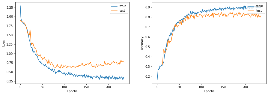
x_test = test_data.paper_id.to_numpy()
_, test_accuracy = gnn_model.evaluate(x=x_test, y=y_test, verbose=0)
print(f"Test accuracy: {round(test_accuracy * 100, 2)}%")
Test accuracy: 82.86%
Conclusion
In this post, we built a GCN node classifier and studied the mathematical foundation behind it. Our GCN network brought in an accuracy of ~83% that is cool. Our major challenge is constructing data for the Graph Neural Network and we simplified that process using an Adjacency Matrix. I am glad I could follow Khalid Salama’s work and reproduce his results, I hope you all enjoyed reading this post.
References
- Node Classification with Graph Neural Networks Khalid Salama, 2021
- Gated Graph Sequence Neural Networks Li, Zemel et al ICLR, 2016
- Simplifying Graph Convolutional Networks Wu, Zhang et al, 2019
- How Powerful Are Graph Neural Networks Xu, Hu et al ICLR, 2019
- Inductive Representation Learning on Large Graphs Hamilton, Ying et al - 2018
- Semi-Supervised Classification With Graph Convolution Networks Kipf and Welling, ICLR - 2017
- Design Space for Graph Neural Networks You, Ying et al, 2021
- A Comprehensive Survey on Graph Neural Networks Wu, Pan et al 2019
- CORA Dataset CORA by Arnaud Barragao