We have studied the Bayesian approach to formulate machine learning models at least a dozen times under the topics uncertainty, density estimation, causality and causal inferences, inductive biases, etc. Previous posts on the Bayesian approach can be read here

• Probabilistic Machine Learning

In this post, we shall revisit the fundamental concepts of the Bayesian approach for building probabilistic machine learning models by establishing an assumption everything is normal and a Gaussian Distribution is a right place to start.

Objective

In this post we shall study the fundamentals of the Bayesian Approach focusing on Gaussian Processes, In that quest, we will be learning the following

• Central limit theorem
• Multivariate Gaussian distributions
• Marginalization and conditioning
• GPs
• Kernels
• Prior and Posterior Dists
• Noise, Uncertainty while Sampling from a GP

Introduction

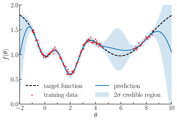
A parametric regression model results in finding a function that represents the prediction line by outputting a set of data points where the residuals are minimized. Whereas, a Gaussian Process is probabilistic that gives confidence measures for the predicted function, i.e, the shaded area in the below plot - a distribution. This distribution has a mean and a standard deviation that represents the most probable characteristics of the data.

• Image Credit: Data-driven Verification and Synthesis of Unknown Systems

Why do we call a Bayesian approach a non-parametric, does that mean we do not consider any predictors(i.e. no data). No, a Bayesian approach presumes there is an infinite number of confounders for a prediction problem and the count of variables grow as the data grows. Hence it is practically impossible to arrive at a full probability model for any problem but we can set a probability function for every problem. Thus comes the Gaussian Process by considering events are normally distributed and their outcomes as well. Few points to remember,

1. Marginal distribution of any subset of elements from multivariabte normal 
distribution is normal
2. Conditional distributions of a subset of elements of a multivariate normal 
distribution are normal

- Chris Fonnesbeck, Vanderbilt University Medical Center.

Central Limit Theorem(CLT):
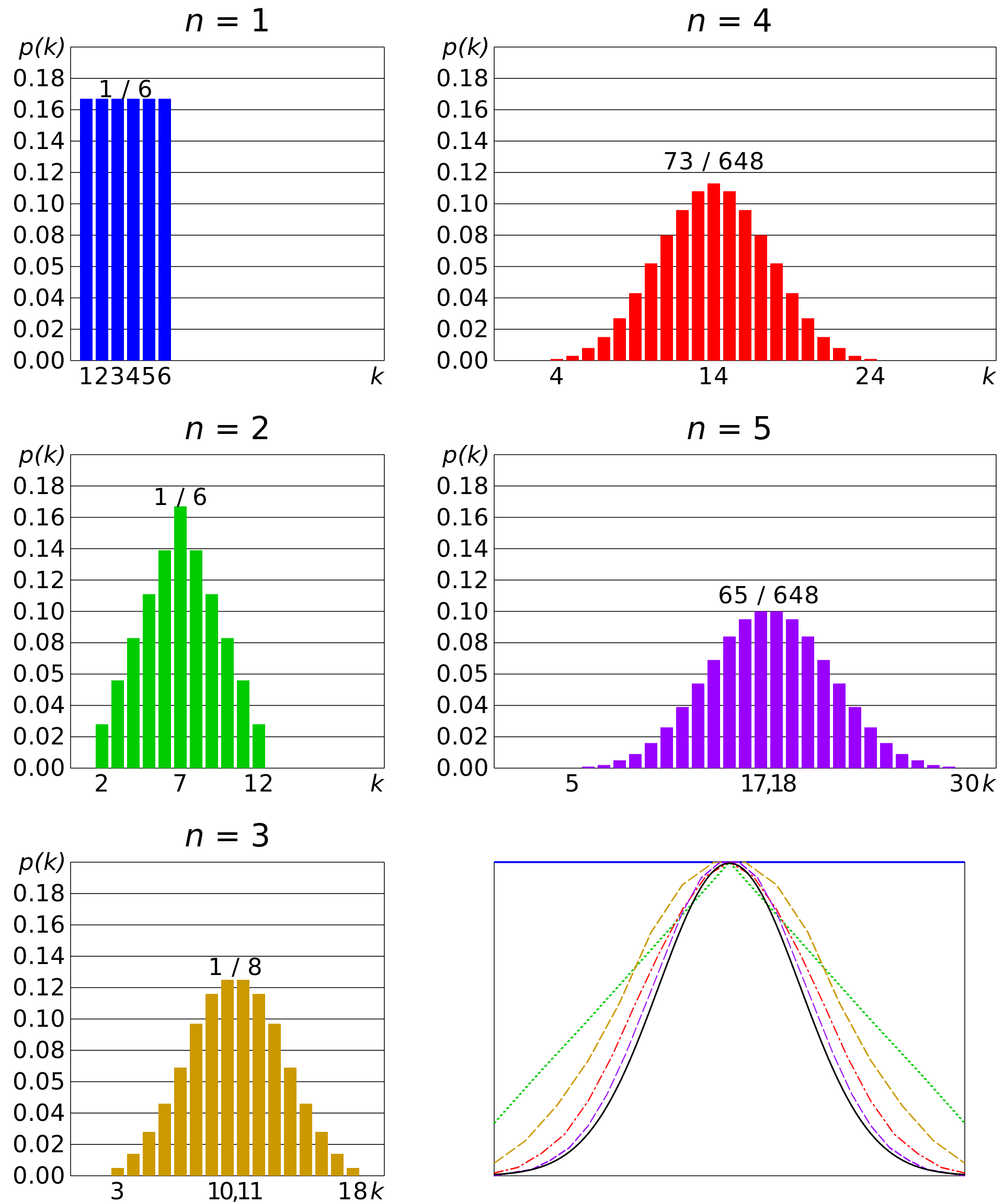
CLT states when the independent random variables are summed up, their sum tends towards a normal distribution. In simple terms, when we roll $n$ unbiased dice of 6 faces the sum of the faces will be approximated to a standard normal distribution(Z). This property is often seen in the real world makes the Gaussian function a valid starting point for identifying the underlying unknown function.

$$Z = lim_{n\rightarrow \infty} \sqrt n\left(\frac{\bar X_n - \mu}{\sigma}\right) \tag{1. Standard Normal Distribution}$$

Where,

• $(X_1, X_2, \cdots, X_n)$ are the random samples

• $\bar X_n$ is the sample mean

• $\sigma$ is the standard deviation

• $\mu$ is the population mean

• 

Properties of Gaussian Processes

We established the intuition behind the influence of infinite confounders for a Bayesian model designing scheme, which naturally leads us to start our study on a multivariate Gaussian distribution. Here each random variable is distributed normally and their joint distribution is also normal. Four properties that we have to consider are

This section is from Cornell Lecture Notes
Refer here

1. Normalization: $\int_y p(y; \mu, \Sigma)dy = 1$
2. Marginalization(Partial Information): The marginal distributions $p(y_A) = \int_{y_B} p(y_A, y_B; \mu, \Sigma)dy_B$ and $p(y_B) = \int_{y_A} p(y_A, y_B; \mu, \Sigma)dy_A$ are Gaussian $$i.e$$ $$y_A \thicksim \mathcal N(\mu_A, \Sigma_{AA})$$ $$y_B \thicksim \mathcal N(\mu_B, \Sigma_{BB})$$
3. Summation If $y \thicksim \mathcal{N}(\mu, \Sigma)$ and $y’ \thicksim \mathcal N (\mu’, \Sigma’)$ then $$y + y’ \thicksim \mathcal{N}(\mu + \mu’, \Sigma + \Sigma’)$$
4. Conditioning(Probability of Dependence): Conditional distribution of $y_A$ on $y_B$ also Gaussian $$p(y_A|y_B) = \frac{p(y_A, y_B; \mu, \Sigma}{\int_{y_A}p(y_A, y_B; \mu, \Sigma)}$$

The above equations demonstrates for 2 variables of $y \rightarrow [y_A, y_B]$, for a multivariate case of $X = [X_1, X_2, \cdots, X_n] \thicksim \mathcal{N}(\mu, \Sigma)$ with a covariance matrix $$\Sigma = Cov(X_i, X_j) = E\left[(X_i - \mu_i)(X_j - \mu_j)^T\right] \tag{2. Covariance Matrix}$$

Gaussian Process

The goal of a GP is to predict the underlying distribution from the dataset. By relooking the properties of the GP, we have the mean$(\mu)$ and the covariance matrix$(\Sigma)$ are our unknowns. Being Gaussian in nature, our first assumption is mean 0 i.e. $\mu = 0$, If $\mu \neq 0$ we can center it once the predictions are made. Now the covariance matrix is left, It determines the shape and characteristics of the unknown distribution.

$$[X_1, X_2, \cdots, X_n] \thicksim \mathcal{N}(0, \Sigma)$$

A GP is a (potentially infinte) collection of random variables (RV) such that the 
joint distribution of every finite subset of RVs is multivariate Gaussian

- Cornell Notes

The covariance matrix is produced by estimating a kernel $k$ function called as covariance function. It receives two points as input and returns a similarity measure between them. $$k: \mathbb{R}^n \times \mathbb{R}^n \rightarrow \mathbb{R}, \Sigma=Cov(X, X’) = k(t, t’)$$ The significance of each entry in a covariance matrix depicts the influence of one point on the other, i.e, the pairwise combination of the $i^{th}$ and $j^{th}$ point for the entry $\Sigma_{ij}$.

Kernels are the methods that measure similarly that goes beyond the euclidean distance. They embed the input points into a higher dimensional space. Few examples of kernels that can be used in a Gaussian process. Kernel functions are of two types

1. Stationary - Functions invariant to translations and the covariance of two points is depend on their relative positions e.g. RBF, Periodic, etc
2. Non-stationary - Depends on their absolute location. e.g, Linear

$$\sigma^2 e^{\left(- \frac {||t -t’||^2}{2l^2}\right)} \tag{3. Radial Basis Fucntion Kernel}$$ $$\sigma^2 e^{\left(- \frac {2sin^2(\pi|t -t’|/p)}{l^2}\right)} \tag{4. Periodic Kernel Fucntion}$$ $$\sigma_b^2 + \sigma^2(t - c)(t’ -c) \tag{5. Linear Kernel Function}$$

Prior and Posterior Distribution

Prior Distribution
We have established a concrete reason for Bayesian inferencing being non-parametric(no data), then the distribution we observe before acquiring any training data is called as prior distribution. That leads to $\mu = 0$ with a covariance matrix of shape $N \times N$. An appropriate kernel function is used to define the covariance matrix.

Posterior Distribution
Once we observe our training data, we can incorporate the infinitely growing information into our Bayesian inferencing model to yield a posterior distribution $P_{X|Y}$. The steps involved are

• Form the joint distribution $P_{X,Y}$ between test points(X) and the training points(Y) $$|Y| + |X| \tag{6. Multivariate Gaussian Distribution}$$
• Used conditioning to find the conditional probability $P_{X|Y}$ from $P_{X,Y}$, conditioning results in derived version of the $\mu$ and the $\sigma$ $$X|Y \thicksim \mathcal{N}(\mu’, \Sigma’) \tag{7. Conditioning}$$

the conditional distribution P_{X|Y} forces the set of functions to precisely pass through each training point. In many cases, this will lead to fitted functions that are 
unnecessarily complex.

-  Görtler et al, Distill.pub

The training points are not perfect measurements. In the real world, the data has noise, errors, and uncertainties due to unknown confounders. To accommodate this, GP provides a mechanism to add the error term $\epsilon \thicksim \mathcal{N}(0, \psi^2)$ to the training points. $$Y = f(X) + \epsilon \tag{8. Error Term}$$

• Image Credit: A Visual Exploration of Gaussian Processes

Marginalization
If we sample at this point, we result in getting a non-deterministic prediction due to the randomness involved in sampling. Using marginalization, a new mean $\mu’$ and corresponding standard deviation $\sigma’$ are for each point is acquired. i.e. $${\mu_1’, \mu_2’, \mu_3’, \cdots, \mu_n’}, {\sigma_1’, \sigma_2’, \sigma_3’, \cdots, \sigma_n’} \thicksim \sigma_i’ = \Sigma_{ii}’ \tag{9. A Bayesian Inference}$$ $$note, \mu \neq 0$$

Conclusion

This post is a revision of the foundational principles of the Bayesian way of looking at the word. The Bayesian approach is quite powerful for the simple reason of being non-parametric, it leads to accommodating infinite parameters during the evolutionary process. My other posts on Bayesian inferencing did not cover the nuances like conditioning and marginalization - results in lack of clarity for someone fresh to Bayesian approach. Please note the critical element of GPs is the measure of uncertainty for the predictions, they also work very well for classification problems along with regression.

References

• A Visual Exploration of Gaussian Processes by Görtler et al at Distill.pub, 2019
• Gaussian process lecture by Andreas Damianou, 2016
• Fitting Gaussian Process Models in Python by Chris Fonnesbeck, 2017
• Machine Learning for Intelligent Systems by Kilian Q. Weinberger
• Central Limit Theorem from Wikipedia
• Estimating Probabilities from data by Kilian Q. Weinberger

gaussian-process-and-related-ideas-to-kick-start-bayesian-inference