In this post, we shall study the mathematical intuition behind Fourier Series for approximating seasonality component for structural time series modeling(STS). This is the second post on STS through Generalized Additive Models(GAMs), we are analyzing the methodologies, evaluation etc briefly in the first part and study Fourier Series in the latter one with a focus on Facebook Prophet. Refer the earlier post on introduction to STS,

• Structural Time Series Models, Why We Call It Structural? A Bayesian Scheme For Time Series Forecasting

• Image Credit: Jean Baptiste Joseph Fourier (1768-1830)

Fourier series could be applied to a wide array of mathematical and physical problems, and especially
those involving linear differential equations with constant coefficients, for which the eigen solutions
are sinusoids.
 - Wikipedia 
 
 

Objective

Objective of this post is to understand periodicity in general and the difference in approach we have to take for Time Series Modeling from conventional ML models by understanding the following topics,

• Single step to multiple time horizons(n-step forecast)
• Moving window approach
• Curve fitting scheme
• Information leak or interpolation
• Forward chaining, Rolling origin
• Naive baselines, 1 Step model and Moving averages
• Seasonal naive baseline
• Evaluation metrics, MAPE to MASE
• Fourier series as arbitrary function of approximation

Further we shall delve into mathematical intuition behind Seasonality approximation using Fourier Analysis.

Introduction

Time series data are analysed at equal time periods, since the challenge is in acquiring data consistently at specified periodicity - It is often aggregated to expected intervals during the pre-processing stage. Modeling often happens at one of the following schemes

1. Single step forecasting - What happens at the next period, for e.g. Forecasting stock price at the next hour
2. Multiple horizon forecasting - What happens at the next n periods, e.g. Stock close price for the next 5 days

• Image Credit Higher Cognition through Inductive Bias, Out-of-Distribution and Biological Inspiration

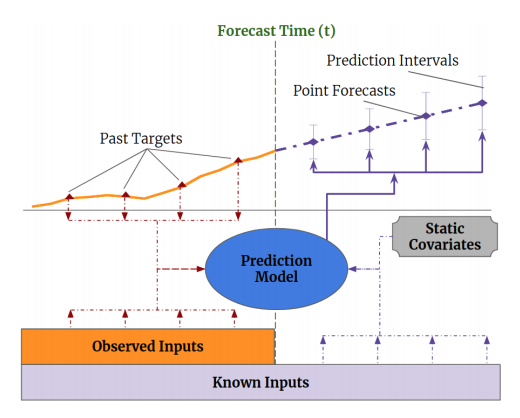
Above diagram renders the scheme of multi-horizon forecasting in purple line.

Moving Window Approach

In this section, we assume the observations are equally spaced for easier understanding of windowing approach. Let us take the example of global gold price aggregated at an hourly space - day close rate and the day(next day) open rate are juxtaposed in the sequence. Caution: this approach does not make much sense if we perceive interval as hour of a day rather than business hours. Meanwhile, a sophisticated approximation function is capable of understanding the hidden domain expertise.

Meanwhile, with windowing approach - Using $n$ observations from the train data - $n+1^{th}$ observation is predicted and evaluated. This scheme is single step forecasting, by moving the window one step ahead ie $t_1, \cdots, t_{n+1}$ one can predict the $t_{n+2}^{th}$ observation. Repeating this process of prediction and evaluation is the scheme of multi horizon forecasting.

• Image Credit Constant-Time Sliding Window Aggregation

Leakage

Data observed as time series are not independent points on the space, they are correlated at time dimension. Hence, we cannot split train, test and validate data like we do conventionally. i.e. In a sequence of data observed at $t_0$ to $t_{25}$, if a random sequence $t_{15}$ to $t_{20}$ split and moved into test set - leakage or interpolation of trend happens backward. This violates the assumption of Independent and Identically Distributed data that we implicitly use in supervised learning. Forward Chaining or Rolling-Origin technique is proposed for cross validation of time series modeling.

We first chunk our data in time, train on the first n chunks and predict on the subsequent chunk, n+1.
Then, we train on the first n+1 chunks, and predict on chunk n+2, and so on. This prevents patterns 
that are specific to some point in time from being leaked into the test chunk for each train/predict 
step.

- Fast Forward Labse of Cloudera

Baselines and Evaluation Metrics

A simple approach to deciding a baseline model is setting the same value observed from the previous time step or crafting moving average(MA) of the window. It is simple and primitive way of defining a baseline but a a good starting point. An improvement can be made with bringing seasonality into account - Seasonal components always makes the model significantly interesting. For example, weather is a major confounder for vegetable harvest - usual weather patterns are of annual cycle and past year yield data will improve the baseline accuracy significantly.

Further, the model performance is calculated and monitored through one or more of the following metrics.

• MAPE: Mean Absolute Percentage Error
• MdAPE: Median Absolute Percentage Error
• sMAPE: Symmetric Mean Absolute Percentage Error
• sMdAPE: Symmetric Median Absolute Percentage Error
• MdRAE: Median Relative Absolute Error
• GMRAE: Geometric Mean Relative Absolute Error
• MASE: Mean Absolute Scaled Error

Seasonality is a key factor in time series model, hence I decided to study Fourier Series as a function of approximation in this post.

• Image Credit: Forecasting at Scale Taylor and Letha of Facebook Prophet team, 2017

The number of events created on Facebook. There is a point for each day, and
points are color-coded by day-of-week to show the weekly cycle. The features of this time
series are representative of many business time series: multiple strong seasonalities, trend
changes, outliers, and holiday effects.

Fourier Series As Function of Approximation

In this section, we study Fourier Series as a periodic function of approximation for seasonality focusing on the architecture of Facebook Prophet. Refer a practical guide on FB Prophet forecasting of NIFTY 50 in one of our earlier posts.

• Is Covid Crisis Lead to Prosperity - Causal Inference from a Counterfactual World Using Facebook Prophet

Overview of GAM

The significance of GAM approach is to achieve easy decomposability and ability to add new components at will. For e.g. When a new factor of seasonality is identified from the observed data, adding it to the model is trivial. Treating forecasting problem as a curve-fitting one accommodates the new sources of information that are identified. This approach inherently promises better interpretability and explanation, which is a boon. It also paves way for analyst in the loop to impose assumptions and presumptions. More about GAMs and STS here.

Seasonality

Machine Intelligence is an idea that strive to understand events and actions that nature exhibits and mimic it when there is a similar stimuli from the environment. Nature demands certain periodic foundations in place that designed our systems to operate in repetitive processes, like

• 5-day work week and a break - to relax and recuperate for the next week, a basic human need
• Fortnight cycle of lunar activity - impacts the tidal energy generation process
• Monthly cycle of accounting activities - lead to seasonal behavior in purchasing power of human beings
• Annual cycle of academic process - result in examinations, new admissions etc

Our quest is to accommodate these natural periodic phenomenons as functions of approximation for attaining convergence.

We rely on Fourier series to provide flexible  model of periodic effects.
- Harvey & Shepard, 1993

Most of the time series data displays the following characteristics,

• Trend
• Seasonality
• Impacts
• Exogenous Variables

$$\Large observation(t) = trend(t) + seasonality(t) + impact(t) + noise \tag{1. Time Series Characteristics}$$

We shall study the mathematical intuition behind seasonality through Fourier Series in the next section.

Fourier Series

The beauty of Fourier Series is its ability to approximate an arbitrary periodic signal, Facebook Prophet taps this idea and generates a partial Fourier sum for standard periods like weekly, daily and yearly.

$$seasonality(t) = \sum_{n=1}^N ( a_n cos ( \frac{2\pi nt}{P} ) + b_n sin(\frac{2\pi nt}{P})) \tag{2.Seasonality Approximation Fourier Function}$$

Where,

• $P$ is the regular period $daily(1), weekly(7), yearly(365.25)$
• $a_n, b_n$ are Fourier coefficients
• $N$ is the number of seasons

$$a_n = \frac{2}{P} \int_P s(x).cos( \frac{2\pi nt}{P} )dt$$ $$b_n = \frac{2}{P} \int_P s(x).sin( \frac{2\pi nt}{P} )dt$$

Our goal is to construct a matrix of seasonality vectors($\beta$) for each value of $t$ in our historical and future data. Then, $$seasonality(t) = X(t)\beta \tag{3. Seasonality}$$ $$where$$ $$\beta = [a_1,b_1 \cdots a_N, b_n]^T$$ $$and$$ $$X(t) = [ cos \frac{ (2\pi (1) t}{365.25}, \cdots, sin \frac{(2\pi(5)t}{365.25}] $$ $$for N = 5$$

Notes:

• $\beta$ is standard normal function with $\mu = 0$ to impose a smoothing prior on the seasonality
• Truncating $N$ applies a low-pass filter $\rightarrow$ increasing $N$ allows for fitting seasonal patterns that change quickly and vise versa
• Prophet team found $N=10$ and $N=3$ as yearly and weekly seasonality count respectively to make most of the problems work

Inference

In this post, we studied mathematical intuition behind Fourier Series as an approximation function for seasonality modeling. Along with approximation function, we understood the nuances in building a time series models like evaluation functions, baseline selection, information leak etc. In the future posts, we shall study the function approximation of trend, events, auto regressive models etc. Until then, Adios Amigos.

References

• Forecasting at Scale Taylor and Letha of Facebook Prophet team, 2017
• Twitter thread on Facebook Prophet Architecture by Sean J. Taylor, 2019
• Structural time series from Cloudera Fast Forward
• Fourier Series from Wikipedia
• Time series Forecasting from Tensorflow
• Another look at measures of forecast accuracy by Hyndman et al, 2005