Continuation of this post:

• That Straight Line Looks a Bit Silly - Let Us Approximate A Sine Wave Using UAT
  Posted November 29, 2021 ‐ 4 min read

By picking Universal Approximation Theorem as the ground topic, we shall study the fundamental concepts of neural networks and progressively enjoy their elegance. This post comes under the subtopic Convergence of Math for AI/ML series, Please refer to the previous articles here,

• Mathematics for AI/ML - Convergence

A feedforward network with a single layer is sufficient to represent 
any function, but the layer may be infeasibly large and may fail to 
learn and generalize correctly.

- Ian Goodfellow

I thank Laura Ruis for writing the post Learning in High Dimension Always Amounts to Extrapolation, It inspired me to write this one. I thank Dr. Anne Hsu for her explanation on UAT - Without her video tutorial, this post wouldn’t have been possible.

Objective

The objective of this post is to understand the Universal Approximation Theorem for Neural Networks and enjoy its beauty. We are writing a few blocks of code to compose this post a visual treat.

Introduction

What makes the neural networks tick is the universality and the learnability. We often focus on the concept of learnability and the learning algorithm but seldom on the underlying universality rule. To get an intuition on what I am talking about, our nature by itself is governed by universal rules and truths like a gravitational pull, escape velocity, etc. Using deep learning models, we are just trying to mimic nature and nature’s phenomenons under a controlled setup. One should never forget, we do not have infinite energy and storage to hold all the confounding factors to make our systems deterministic. Hence, we are building a stochastic network of systems by approximating the outcomes for a given set of inputs.

Karen Kao: You think deep learning will be enough to replicate all of 
human intelligence. What makes you so sure?

Dr. Geoffrey Hinton: I do believe deep learning is going to be 
able to do everything, but I do think there’s going to have to be 
quite a few conceptual breakthroughs. For example, in 2017 Ashish 
Vaswani et al. introduced transformers, which derive really good 
vectors representing word meanings. It was a conceptual 
breakthrough.

- Conversation between Dr. Hinton and Karen Kao, 
    MIT Technology Review, Nov, 2020

• Image Credit: Can neural networks solve any problem? by Brendan Fortuner

Let us say we have a continuous function $f(x)$ for which we would like to build a model that approximates the outcomes for any given input value of $x$. We shall call the output function as $g(x)$ Then,

$$|f(x) - g(x)| < \epsilon \tag{1. Objective Function}$$

Where, $\epsilon$ is the error that we intend to minimize or in other words - the objective of our deep learning model. $\epsilon$ decides the precision of the approximations made by the model.

A Single Neuron

The basic unit of a Neural Network is its Neuron, also called perceptrons. We shall take this opportunity to describe how a neuron from a neural network is metaphorical to a biological neuron. For simplicity, we shall assume the neuron of our interest is connected to only one neuron to feed the input. i.e Inputs are fed into our neuron that traveled across the axon of the previous neuron through a synaptic connection via a Dendrite. A deeper understanding can be obtained of the biological point of view from the below 2 posts.

• With 20 Watts, We Built Cultures and Civilizations - Story of a Spiking Neuron
• Understanding Post-Synaptic Depression through Tsodyks-Markram Model by Solving Ordinary Differential Equation

What’s inside the brain is these big vectors of neural activity.

- Dr. Geoffrey Hinton, 2020

import numpy as np
import matplotlib.pyplot as plt

# f(x)
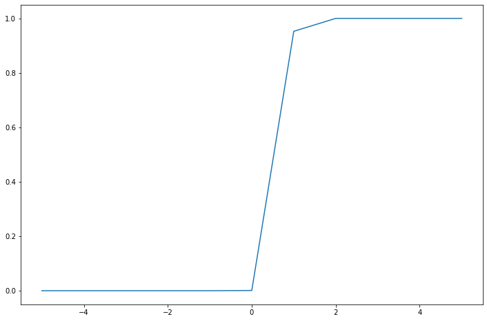
f = lambda a, w, b: w * a + b
# activation function
sigmoid = lambda z: 1. / (1 + np.exp(-z))

x = np.array([-5, -4, -3, -2, -1, 0, 1, 2, 3, 4, 5])
w = 10
b = -7

y = sigmoid(f(x, w, b))
y
plt.figure(figsize=(12, 8))
plt.plot(x, y)

[<matplotlib.lines.Line2D at 0x7ff25cb87dc0>]

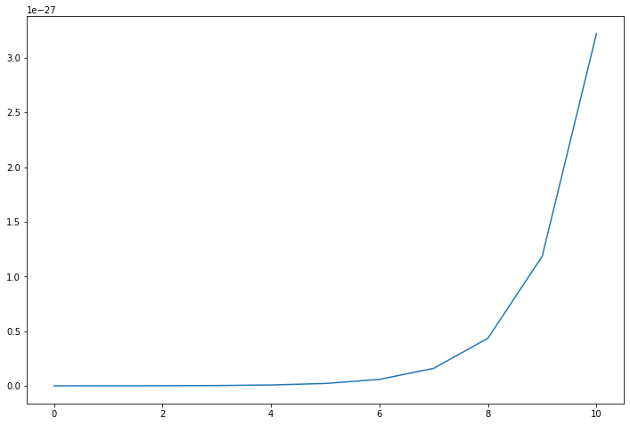
When there are more than one input, i.e there are more neurons connected to our neuron then the scheme looks as follows. For simplicity we shall restrict the input count to 3 and build the function $f(x)$

b = -7
x1 = np.array([-5, -4, -3, -2, -1, 0, 1, 2, 3, 4, 5])
w1 = 10

x1w1 = f(x1, w1, b)

x2 = np.array([0, 1, 2, 3, 4, 5, 6, 7, 8, 9, 10])
w2 = -2

x2w2 = f(x2, w2, b)

x3 = np.array([0, -1, -2, -3, -4, -5, -6, -7, -8, -9, -10])
w3 = 7

x3w3 = f(x3, w3, b)

y = sigmoid(x1w1 + x2w2 + x3w3)
plt.figure(figsize=(12, 8))
plt.plot(np.arange(11), y)

[<matplotlib.lines.Line2D at 0x7ff25d1062b0>]

That is how a typical neuronal activation happens in complex neural networks. To make our life easier, we shall simplify the problem further by building a neural network with a step activation function.

Binary Step Activation Function

A binary step activation function is the simplest activation function where the neuron gets activated when the input crosses a threshold value. i.e $$f(x) = 1, if x \geq T$$ $$f(x) = 0, if x < T$$ Where, $T$ is certain threshold.

Let us build the neuron portrayed in this picture. As mentioned, the neuron takes 3 items as input,

1. The input vector $x_i$
2. The weights $w_i \thicksim w$ - to simplify we are going to take the same weight
3. The bias $b$

There are two lambda functions we are building,

1. The Weights and Biases $f$ depicted as the yellow region in the neuron architecture
2. The STEP activation function $step$ depicted as the purple region in the neuron architecture

def neuron(inputt, weight, bias):
    # Yellow Region
    f = lambda a, w, b: w * a + b
    # Purple Region
    step = lambda a, T: T if a >= T else 0

    f_of_x = f(inputt, weight, bias)
    output = [step(an_item, T) for an_item in f_of_x]

    return f_of_x, output

Help functions to plot the neuron activations.

# Help functions to plot the graphs
def plot_steps(inputt, f_of_x, output, color, ax, title, label):
    ax.plot(inputt, f_of_x, color="green", label=f"f(x) = $\sum_i w_i x_i + bias$")
    ax.step(inputt, output, color=color, alpha=0.8, label=label)
    ax.set_title(title)
    ax.legend()
    ax.grid(True, which='both')
    ax.axhline(y=0, color='black', linewidth=4, linestyle="--")
    ax.axvline(x=0, color='black', linewidth=4, linestyle="--")

import matplotlib.image as mpimg
def render_image(ax, image_file):
    img = mpimg.imread(image_file)
    ax.imshow(img)

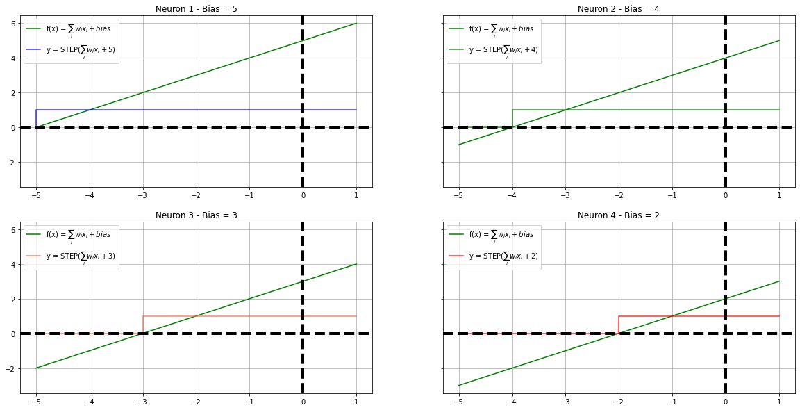
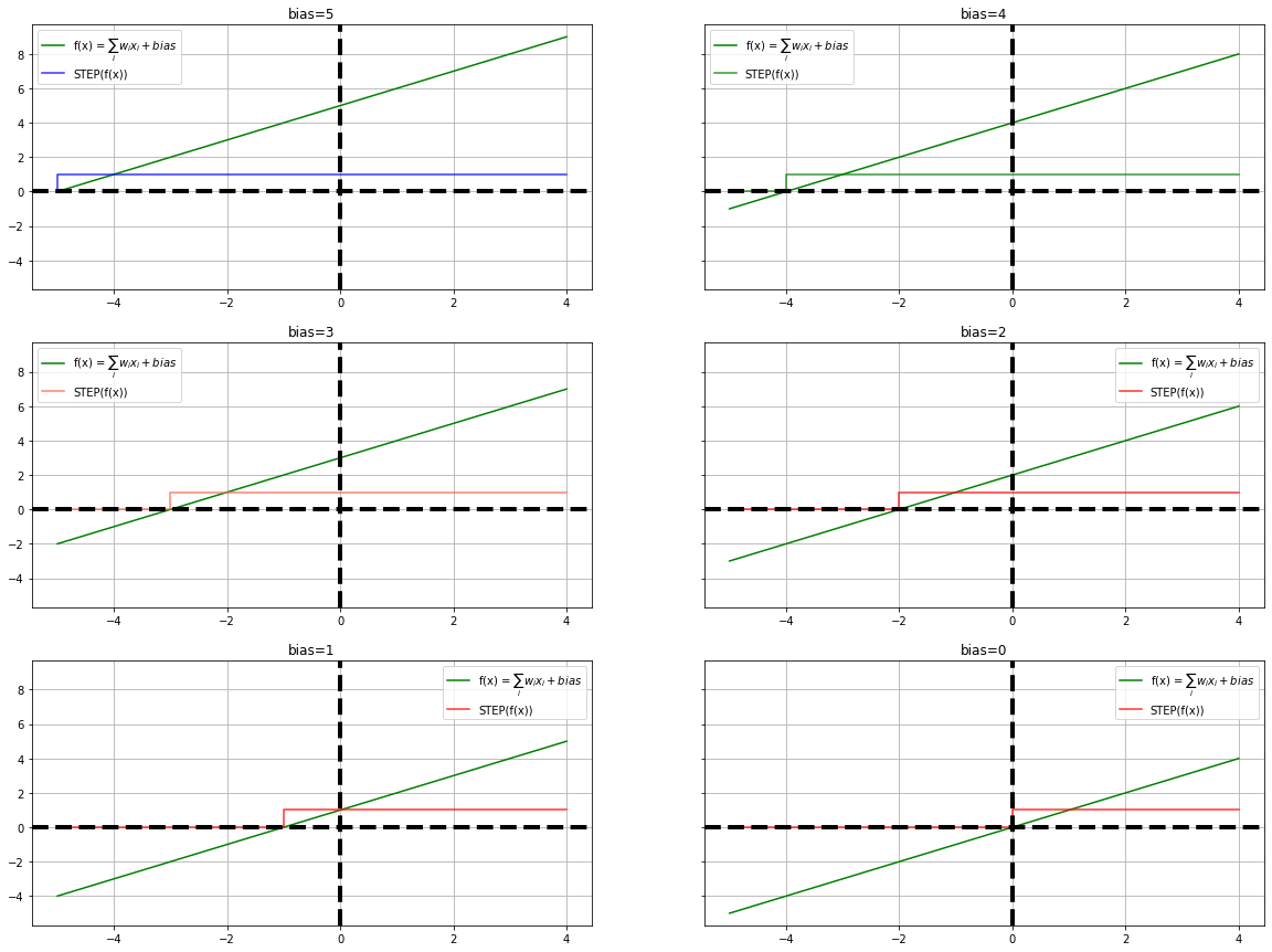
We shall build 4 neurons with varying biases to demonstrate the effect of the activation. Please note, we are having constant weight across all the neurons for easy understanding and the threshold of the step function is 1, ie. It operates at the region $0 - 1$

x = np.arange(-5, 2, 1)
plt.figure(figsize=(12, 8))
fig, ([[ax1, ax2], [ax3, ax4]]) = plt.subplots(2, 2, figsize=(20, 10), sharey=True)

b = 5
w = 1
T = 1
fx1, y1 = neuron(x, w, b)
plot_steps(x, fx1, y1, "blue", ax1, "Neuron 1 - Bias = 5", label=f"y = STEP($\sum_i w_i x_i + {b}$)")

b = 4
w = 1
T = 1

fx2, y2 = neuron(x, w, b)
plot_steps(x, fx2, y2, "green", ax2, "Neuron 2 - Bias = 4", label=f"y = STEP($\sum_i w_i x_i + {b}$)")

b = 3
w = 1
T = 1

fx3, y3 = neuron(x, w, b)
plot_steps(x, fx3, y3, "tomato", ax3, "Neuron 3 - Bias = 3", label=f"y = STEP($\sum_i w_i x_i + {b}$)")

b = 2
w = 1
T = 1

fx4, y4 = neuron(x, w, b)
plot_steps(x, fx4, y4, "red", ax4, "Neuron 4 - Bias = 2", label=f"y = STEP($\sum_i w_i x_i + {b}$)")

<Figure size 864x576 with 0 Axes>

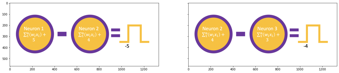
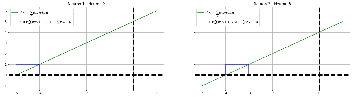
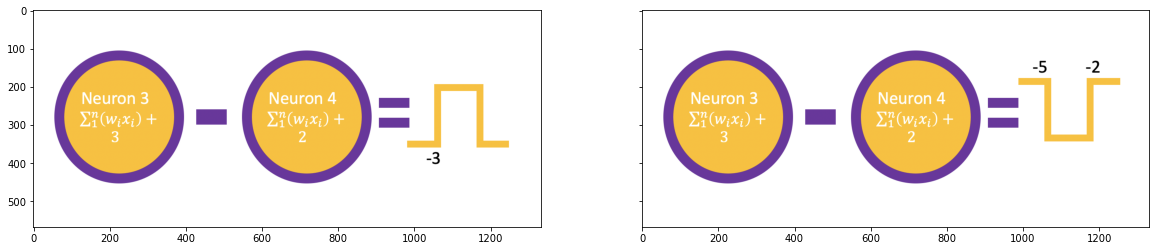
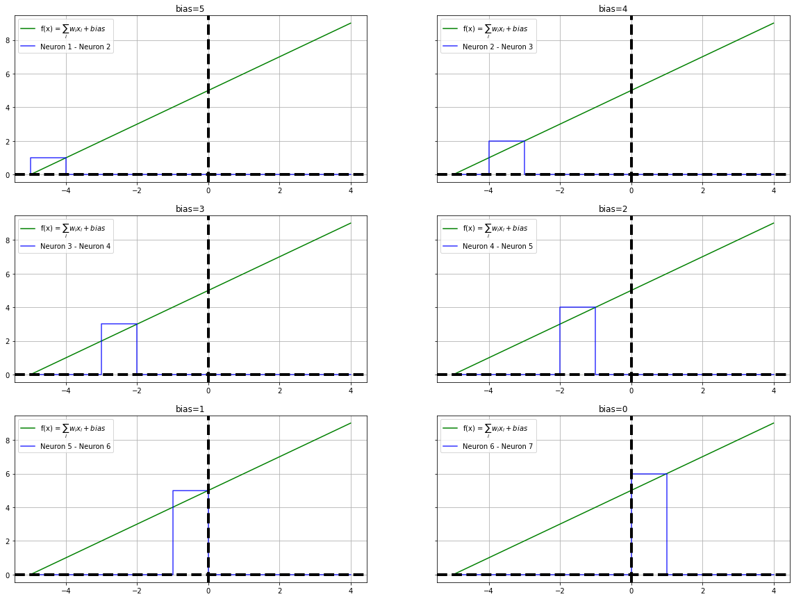
The four neurons we have constructed are juxtaposed with each other to form a circle and their interactions are calibrated. i.e The difference between adjacent neuronal output is calculated to simulate a step function. For recreational and educational purposes, we are placing the last neuron and the first neuron next to each - This scheme will demonstrate a critical behavior of the neural network.

y12 = list(np.array(y1) - np.array(y2))
y23 = list(np.array(y2) - np.array(y3))
y34 = list(np.array(y3) - np.array(y4))
y41 = list(np.array(y4) - np.array(y1))

fig, ([ax1, ax2]) = plt.subplots(1, 2, figsize=(20, 5), sharey=True)
render_image(ax1, "n12.png")
render_image(ax2, "n23.png")

fig, ([ax1, ax2]) = plt.subplots(1, 2, figsize=(20, 5), sharey=True)
plot_steps(x, fx1, y12, "blue", ax1, "Neuron 1 - Neuron 2", label=f"STEP($\sum w_ix_i + 5$) - STEP($\sum w_ix_i + 4$)")
plot_steps(x, fx2, y23, "blue", ax2, "Neuron 2 - Neuron 3", label=f"STEP($\sum w_ix_i + 4$) - STEP($\sum w_ix_i + 3$)")
fig, ([ax1, ax2]) = plt.subplots(1, 2, figsize=(20, 5), sharey=True)
render_image(ax1, "n34.png")
render_image(ax2, "n41.png")
fig, ([ax1, ax2]) = plt.subplots(1, 2, figsize=(20, 5), sharey=True)
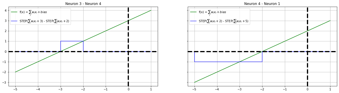
plot_steps(x, fx3, y34, "blue", ax1, "Neuron 3 - Neuron 4", label=f"STEP($\sum w_ix_i + 3$) - STEP($\sum w_ix_i + 2$)")
plot_steps(x, fx4, y41, "blue", ax2, "Neuron 4 - Neuron 1", label=f"STEP($\sum w_ix_i + 2$) - STEP($\sum w_ix_i + 5$)")

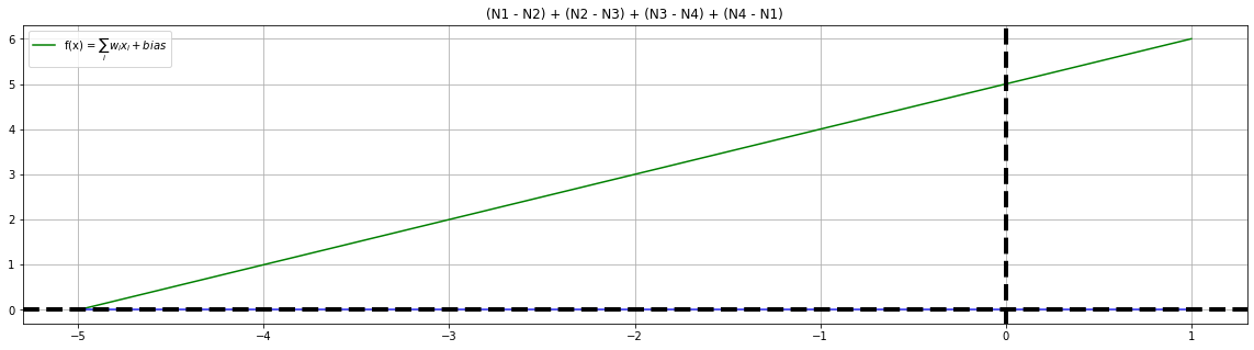
Tail Function

A tail function is an aggregator of all the neuronal outputs from the hidden layer, here we are adding any biases but adding the outcomes of the hidden layer.

Unsurprisingly, the effect of Fist and Fourth neuron pair cancels out all the activations gives us a food for thought.

fig, ax = plt.subplots(1, 1, figsize=(20, 5), sharey=True)
y = list(np.array(y12) + np.array(y23) + np.array(y34) + np.array(y41))
plot_steps(x, fx1, y, "blue", ax, f"(N1 - N2) + (N2 - N3) + (N3 - N4) + (N4 - N1)", label="")

Universal Approximation Theorem - Implementation

In this section, we shall combine them all and see how the final result looks. Our objective is to bring in the steps that follow the $f(x)$. These steps are the outcome of the intended $g(x)$ function we discussed in the introduction.

x = np.arange(-5, 5, 1)
plt.figure(figsize=(20, 15))
fig, ([[ax1, ax2], [ax3, ax4], [ax5, ax6]]) = plt.subplots(3, 2, figsize=(20, 15), sharey=True)
b1 = 5
w1 = 1
T = 1
fx1, y1 = neuron(x, w1, b1)
plot_steps(x, fx1, y1, "blue", ax1, title=f"bias={b1}", label=f"STEP(f(x))")

b2 = 4
w2 = 1
T = 1

fx2, y2 = neuron(x, w2, b2)
plot_steps(x, fx2, y2, "green", ax2, title=f"bias={b2}", label=f"STEP(f(x))")

b3 = 3
w3 = 1
T = 1

fx3, y3 = neuron(x, w3, b3)
plot_steps(x, fx3, y3, "tomato", ax3, title=f"bias={b3}", label=f"STEP(f(x))")

b4 = 2
w4 = 1
T = 1

fx4, y4 = neuron(x, w4, b4)
plot_steps(x, fx4, y4, "red", ax4, title=f"bias={b4}", label=f"STEP(f(x))")

b5 = 1
w5 = 1
T = 1

fx5, y5 = neuron(x, w5, b5)
plot_steps(x, fx5, y5, "red", ax5, title=f"bias={b5}", label=f"STEP(f(x))")

b6 = 0
w6 = 1
T = 1

fx6, y6 = neuron(x, w6, b6)
plot_steps(x, fx6, y6, "red", ax6, title=f"bias={b6}", label=f"STEP(f(x))")

b7 = -1
w7 = 1
T = 1

fx7, y7 = neuron(x, w7, b7)

<Figure size 1440x1080 with 0 Axes>

y12 = list(np.array(y1) -  np.array(y2))
y23 = list(2 * (np.array(y2) -  np.array(y3)))
y34 = list(3 * (np.array(y3) - np.array(y4)))
y45 = list(4 * (np.array(y4) - np.array(y5)))
y56 = list(5 * (np.array(y5) - np.array(y6)))
y67 = list(6 * (np.array(y6) - np.array(y7)))

fig, ([[ax1, ax2], [ax3, ax4], [ax5, ax6]]) = plt.subplots(3, 2, figsize=(20, 15), sharey=True)

plot_steps(x, fx1, y12, "blue", ax1, title=f"bias={b1}", label=f"Neuron 1 - Neuron 2")
plot_steps(x, fx1, y23, "blue", ax2, title=f"bias={b2}", label=f"Neuron 2 - Neuron 3")
plot_steps(x, fx1, y34, "blue", ax3, title=f"bias={b3}", label=f"Neuron 3 - Neuron 4")
plot_steps(x, fx1, y45, "blue", ax4, title=f"bias={b4}", label=f"Neuron 4 - Neuron 5")
plot_steps(x, fx1, y56, "blue", ax5, title=f"bias={b5}", label=f"Neuron 5 - Neuron 6")
plot_steps(x, fx1, y67, "blue", ax6, title=f"bias={b6}", label=f"Neuron 6 - Neuron 7")

y = list(np.array(y12) + np.array(y23) + np.array(y34) + np.array(y45) + np.array(y56))
fig, ax = plt.subplots(1, 1, figsize=(10, 5), sharey=True)
plot_steps(x, fx1, y, "blue", ax, title="A", label="B")

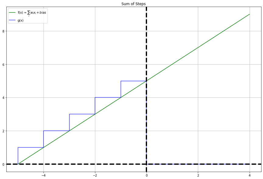
Conclusions

In this post, we studied the Universal Approximation Theorem with a few assumptions and presumptions. The key learning is with one hidden layer we can approximate a leading straight line quite intuitively with a visual treat. This simple but powerful concept is the reason we can achieve convergence in deep learning systems. For simplicity, I kept the weights constant and varying biases - This approach helped me to get to the critical aspect of UAT easily. Weights and biases are the learning parameters of a deep learning model, One of my earlier posts intuitively details the same idea. Please refer it here,

• Automatic Differentiation Using Gradient Tapes

Hope you enjoyed this post and I am saying goodbye until another post.

References

• The Universal Approximation Theorem for neural networks by Michael Nielsen, 2017
• AI pioneer Geoff Hinton: “Deep learning is going to be able to do everything by Conversation with Dr. Hinton, MIT Review, 2020
• 03 Intro to Deep Learning Part3: Universal Approximation Theorem by Dr. Anne Hsu, 2020
• Deep Learning with Python, 2nd Edition by François Chollet, 2020
• A visual proof that neural nets can compute any function by Michael Nielsen, 2019
• Can neural networks solve any problem? by Brendan Fortuner, 2017
• Power of a Single Neuron by Vaibhav Sahu, 2018
• Getting to know Activation Functions in Neural Networks by Hasara Samson, 2020

# do-you-know-we-can-approximate-any-continuous-function-with-a-single-hidden-layer-neural-network-a-visual-guide