Cocktail Party Problem - Eigentheory and Blind Source Separation Using ICA
Posted July 18, 2021 by Gowri Shankar ‐ 13 min read
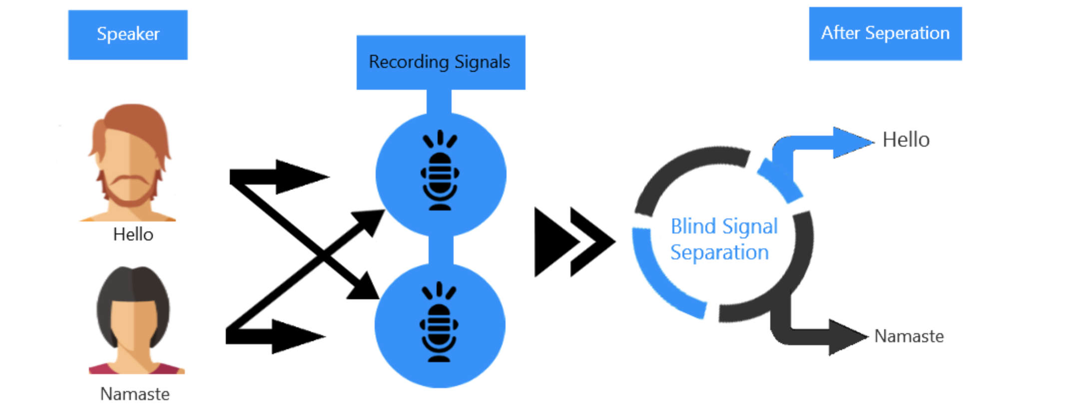
We will never achieve 100% accuracy on our predictability of real world events using any AI/ML algorithm and accuracy is a one simple metric that always lead to deception, Why? Data observed from the nature is always a mixture of multiple distinct sources, separating them by their origin is the basis for understanding. The process of separating the signals that consummate an observed data is called Blind Source Separation. Pondering, we human beings are creatures of grit and competence to come up with techniques like Independent Component Analysis(ICA) in the quest for understanding the complex entities of nature.
Blind source separation of complex datasets are intractable beacuse of the challenges in distinct identification of independent sources along with the noises and fluctuationss. In this post, we shall explore the mathematical intuition behind a naive but important technique called independent component analysis on a sophisticated signal. ICAs are widely used in signal processing, image processing especially medical images and audio signals. Another related topic of interest is Principal Component Analysis that was studied in another post earlier, Please refer… -Eigenvalue, Eigenvector, Eigenspace and Implementation of Google’s PageRank Algorithm
Trivia
- BSS/ICA are not new topics, they first appeared in 80s but ignored due to the excitement and drumbeat caused by backpropagation algorithm.
- This post is a walk through of Jonathan Schlens paper on Blind Source Separation
- I confess, there are ambiguity in this post - It is a brave attempt from my end on a topic that pushed me to think beyond my comprehension
- This post covers a handful number of topics that I truly love - eigentheory, entropy etc are to name a few.
- Image Credit: Blind Source Separation for Cocktail Party Problem
Objectives
This post is a mere summary of Jonathon Shlens un-scholarly(he claims) paper titled A Tutorial on Independent Component Analysis, I tried my best to understand every nuances of blind source separation through ICA but I confess I have to go a long way to realize a tangible work-product out of this study.
Prologue
Though there are so many things that caused nightmares about this topic, 3 topics pushed me to take a plunge,
- My love for eigenvalues, eigenvectors and eigenspaces
- Entropy, the measure of uncertainty and
- The quest for understanding the nature by understanding the data that we collect from the nature - through blind source separation.
This post is organized as follows,
- There are 3 sections in this post,
- Elaborates the problem
- Explores the unknowns and cleverly simplifies an under-constrained problem
- Measures the single unknown using the principles of information theory
Further elaborating the content of each sections below,
- Section 1: Introduction
- Introduces signals of multiple sources
- Explains linear mixture of signals through cocktail party problem
- Mathematical intuition behind ICA
- Mixing matrix the linear mixture of indedpendent sources
- Simplify the problem using singular value decomposition to identify the unknowns
- Section 2: Solving the Unknowns
- Explores the significance of covariance matrix
- Covariance of independent sources
- Decomposing an arbitrary matrix using orthogonal diagonalization
- Reconstruction of mixing matrix
- Whitening the observed data through rotation and and normalization
- Intuition behind statistical independence and factorial distributions
- Section 3: Measuring Independence
- Concepts of information theory: Mutual Information, Multi Information etc
- Entropy, measure of uncertainty
- Minimizing multi-information to find the rotation matrix
Introduction
Richard Feynnman once said, “If you can’t explain something in simple terms, you don’t understand it”. This quote is quite apt for the challenges we face in XAI, One that is understood is explainable, One that is explainable is measurable, Only those that are measurable are monitored and improved. Though we measure the model performances through various metrics (e.g. accuracy, loss etc) we never achieve the absolute convergence because of 2 reasons,
- Corruption of observations due to random noise
- Measurements are often the linear sum of multiple sources
In this post, we shall explore the cases where the measurements are combination(or linear sum) of multiple sources. For e.g. audio signals are the classic examples of linear mixture of multiple sources.
Let us take the case of Cocktail Party Problem - Two sound sources $s_1$ and $s_2$ are generated by music and voice, recorded simultaneously from two different microphones.
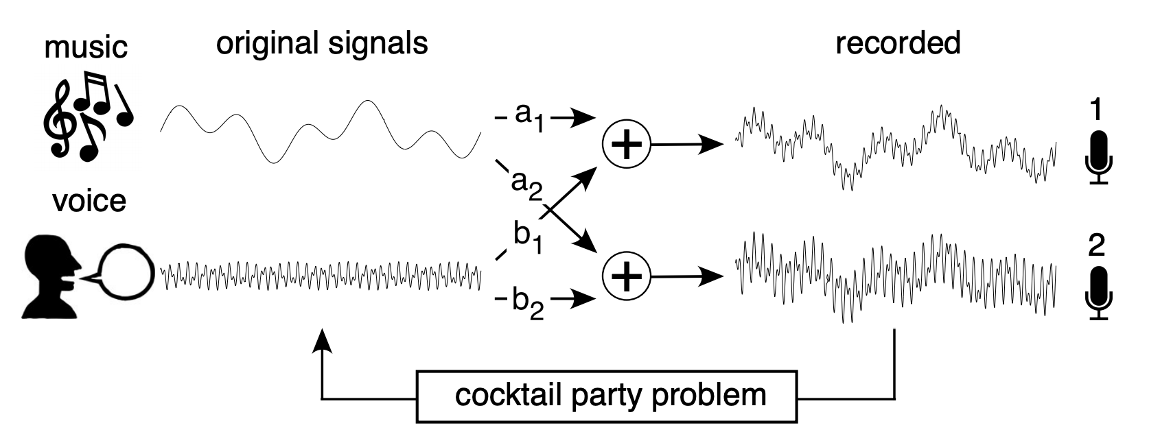
- Image Credit: A Tutorial on Independent Component Analysis
The proximity of each speaker to their respective microphones are incorporated as linear weights${(a_1, a_2), (b_1, b_2)}$ for each microphones and goal of the problem is to recover the original sources from the recordings.
Similarly, blurry images captured due to motion in the camera when the camera aperture is open - an example for linear sum of multiple sources. Here, first source is the original image and the second source is camera motion trajectory. De-blurring the corrupted image to recover the original one is the goal.
Linear Mixture Problem When the combination of two signals results in the superposition of signals, we term this problem a linear mixture problem.
– Jonathan Schlens, Google Research
ICA - The Problem Definition
ICA is a statistical and computational technique that reveals the underlying set of random variables, measurements or signals from an observed multivariate dataset. ICA separation process of a complex linearly mixed signal works well if the source signals are
- Independent of each other
- Not normally distributed(non-gaussian)
Few observations,
- though the source signals are independent; their mixtures are not necessarily independent.
- Mixture of independent signals tend to get closer to a Gaussians of high temporal complexity.
Given a set of observations ${ x_1(t), x_2(t), x_3(t), \cdots, x_n(t) }$ where $t$ is the index of the sample(time), then a linear mixture model of independent components can be written as
$$\Large \mathbf{x} = \mathbf{A}\mathbf{s} \tag{1. Linear Mixture}$$ Where,
- $\mathbf{A}$ is an unknown invertible, square matrix that mixes the components of the sources
- $\mathbf{s} = { s_1(t), s_2(t), s_3(t), \cdots, s_n(t) }$ are the independent sources
In our cocktail party problem $s_1(t)$ is music and $s_2(t)$ is voice.
For clarity, the linear mixing matrix A for the cocktail party problem depicted in the picture is
$$\mathbf{A} = \left( \begin{array}{cc} a_1 & b_1 \ a_2 & b_2 \end{array} \right) \tag{2. Mixing Matrix}$$
Our goal is to solve for the matrix $A$, rather $A^{-1}$, i.e. from $eqn.1$ $$\mathbf{s} = \mathbf{A}^{-1}\mathbf{x}$$ Since this is an approximation problem, we shall rewrite the equation as follows. $$\Large \hat {\mathbf{s}} = \mathbf{W}\mathbf{x} \tag{3. Approximation}$$
It is an under-constrained problem because we have two unknows $\hat s$ and $W$ and one known $x$. i.e the total number of unknowns are more than the number of knowns.
Decomposition of Mixing Matrix
Our approach is to solve for $\mathbf{A}$ by cutting up $\mathbf{A}$ into simpler and more manageable parts using Singular Value Decomposition(SVD). SVD is a linear algebra technique that provides method for dividing $\mathbf{A}$ into several smaller pieces. Any arbitrary matrix can be decomposed into 3 linear operations
- A rotation $\mathbf{V}$
- A Stretch $\sum$ and
- A second roation $\mathbf{U}$ $$\mathbf{A} = \mathbf{U} \Sigma \mathbf{V}^T \tag{4. Decomposition}$$ $$i.e.$$ $$\Large \mathbf{W} = \mathbf{A}^{-1} = \mathbf{V} \Sigma ^{-1} \mathbf{U}^T \tag{5. Decomposition of Approximation}$$
Inverse of a rotation matrix is its transpose, i.e $\mathbf{V}^{-1} = \mathbf{V}^T$
- We shall examine the covariance of the data observed $\mathbf{x}$ to calculate $\mathbf{U}$ and $\Sigma$
- Assumption of independence of $\mathbf{s}$ to solve for $\mathbf{V}$
Solving for $U, V \ and \ \Sigma$
The significance of the covariance matrix is it measures all correlations that can be captured by a linear model, being the appropriate starting point for solving our unknowns. Covariance also the expected value of the outer product of individual data points $[\mathbf{x}\mathbf{x}^T]$. From $eqn.1$ $\mathbf{x} = As$
$$(\mathbf{x}\mathbf{x}^T) = [(\mathbf{As})(\mathbf{As})^T]$$ $$(\mathbf{x}\mathbf{x}^T) = [(\mathbf{U} \Sigma \mathbf{V}^Ts)(\mathbf{U} \Sigma \mathbf{V}^Ts)^T]$$ $$(\mathbf{x}\mathbf{x}^T) = \mathbf{U} \Sigma \mathbf{V}^T [\mathbf{s}\mathbf{s}^T] \mathbf{V} \Sigma \mathbf{U}^T $$
We know $\mathbf{s}\mathbf{s}^T = \mathbf{I}$, then $$\Large (\mathbf{x}\mathbf{x}^T) = \mathbf{U} \Sigma^2 \mathbf{U}^T \tag{6. Covariance is Independent of Sources}$$
$eqn.6$ depicts
- Covariance of the data is independent of sources $\mathbf{s}$ and $\mathbf{V}$.
- Expressing covariance in terms of diagonal matrix $\Sigma^2$ between 2 orthogonal matrices $\mathbf{U}$
Orthogonal Diagonalization
Orthogonal diagonalization is a decomposition operation of converting any arbitrary matrix $\mathbf{A}$ into a diagonal matrix by multiplying by an orthogonal basis. Orthogonal diagonalization is achieved by an orthogonal basis of eigenvectors stacked as columns and a diagonal matrix composed of eigenvalues. Refer, -Eigenvalue, Eigenvector, Eigenspace and Implementation of Google’s PageRank Algorithm
Consider a matrix $\mathbf{E}$ whose columns are eignevectors of the covariance of our dataset. We can prove, $\mathbf{D}$ is a diagonal matrix of associated eigenvalues. The eigenvectors of the covariance of the data form an orthonormal basis meaning that $\mathbf{E}$ is an orthogonal matrix.
$$\Large (\mathbf{x}\mathbf{x}^T) = \mathbf{ED} \mathbf{E}^T \tag{7. Orthogonal Diagonalization}$$
Analysizng $eqn.6 \ and \ eqn.7$
- Both the equations states that the covariance of the data can be diagonalized by an orthogonal matrix
- $eqn.4$ provides a decomposition based on the assumption of ICA
- $eqn.5$ provides decomposition based on the properties of symmetric matrices
- Diagonalizing a symmetric matrix using eigenvectors is a solution up to a permutation, no other basis can diagonalize a symmetric matrix
Solution for $\mathbf{U}$ and $\Sigma$ Hence, if our assumptions for ICA are true - We have a partial solution for $\mathbf{A}$.
- $\mathbf{U}$ is a matrix of the stacked eigenvectors of the covariance of our dataset.
- $\Sigma$ is a diagonal matrix with the square root of the associated eigenvalue in the diagonal.
With those intuitions in place, from $eqn.5$, $\mathbf{W}$ is constructed as follows. $$\Large \mathbf{W} = \mathbf{VD}^{-\frac{1}{2}}E^T \tag{8. Reconstructed Mixing Matrix}$$ Where,
- $\mathbf{D} \ and \ \mathbf{E}$ are eigenvalues and eigenvectors of the covariance of the dataset $\mathbf{x}$
- $\mathbf{V}$ is the only unknown rotation matrix
Whitening: Map Data To Spherically Symmetric Distribution
Whitening removes all linear dependencies in a dataset and normalizes the variance along all dimensions, intuitively this operation maps the dataset into a spherically symmetric distribution. i.e from $eqn.8$
$$\Large \underbrace{ \mathbf{D}^{-\frac{1}{2}} }{\text{STEP 2 -}}\underbrace{E^T}{\text{STEP 1}}$$
STEP 1: Rotate to align with eigenvectors $E^T$
- Multiplying $\mathbf{E}^T$ performs the rotation to decorrelate the data by removing linear dependencies.
- Decorrelation means that the covariance of the transformed data is diagnolized
- $\mathbf{D}$ is a diagonal matrix of the eigenvalues, i.e. each entry in $\mathbf{D}$ is an eigenvalue of the covariance of the transformed data. This is nothing but Principal Component Analysis(PCA).
- Projecting a dataset onto a principal components removes linear correlations and provide a strategy for dimensional reduction.
From $eqn.7$ $$\Large (\mathbf{x}\mathbf{x}^T) = \mathbf{ED} \mathbf{E}^T$$ $$\mathbf{E}^T [\mathbf{x}\mathbf{x}^T] \mathbf{E} = \mathbf{D}$$ $$[\mathbf{E}^T \mathbf{x}\mathbf{x}^T \mathbf{E}] = \mathbf{D}$$ $$[(\mathbf{E}^T \mathbf{x})(\mathbf{E}^T \mathbf{x})^T] = \mathbf{D}$$
STEP 2: Normalization
- Multiplying $\mathbf{D}^{-\frac{1}{2}}$ normalizes the variance in each dimension
- Normalization ensures that all dimensions are expressed in standard units
- No preferred direction exist and the data is rotationally symmetric - like a sphere
Then the whitened dataset is defined as follows $$\Large \mathbf{x}_w = (\mathbf{D}^{-\frac{1}{2}}E^T)\mathbf{x} \tag{9. Whitened Data}$$
Substituting the above equation in $eqn.5$ and $eqn.4$, $\hat {\mathbf{s}} = \mathbf{Vx}_w$. The problem simplifies to find the rotation matrix $\mathbf{V}$.
The Statistics of Independence
If two random variables a and b are independent, then the joint probability factorizes to $P(a, b) = P(a)P(b)$. As per our initial assumption, all sources of an ICA dataset are statistically independent, their joint probablity distribution is
$$\Large \mathbf{P(s)} = \Pi_i \mathbf{P(s_i)} \tag{10. Factorial Distribution}$$
This is a special family of distribution called factorial distribution because the joint distribution is the product of the distribution of each source $\mathbf{s}$.
The problem of ICA searches for the rotation $\mathbf{V}$ such that all sources are statistically independent. All second order correlations are removed and the unknown matrix $\mathbf{V}$ must remove all higher-order correlations. To achieve this we need a function termed as contrast function that meaures the amount of higher order correlations - In other words, measures how close the estimated sources are to statistical independence.
Measuring Statistical Independence
Our goal is to find how close a distribution is to statistical independence, lead to finding out the rotation matrix $\mathbf{V}$. We rely on information theory, a branch of mathematics deals with contrast functions that identifies correlations and approximations to measuring statistical independence.
- Mutual Information: Measures the departure of two variables from statistical independence
- Multi Information $I(y)$: A generalization of mutual information, measures the statistical dependence between multiple variables.
$I(y)$ is a non-negative quantity, It reaches it’s minimum to zero when all its variables are statistically independent.
$$\Large I(y) = \int P(y) log_2 \frac {P(y)}{\Pi_i P(y_i)}dy \tag{11. Mutual Information}$$ $$if$$ $$P(y) = \Pi_i P(y_i) $$ $$then$$ $$\Large log(1) = 0 \rightarrow I(y) = 0$$ $$i.e.$$ $$\text{find a rotation matrix } \mathbf{V} \text{ such that } I(\hat s) = 0 \ where \ \hat s = Vx_w$$
From eqn.8 $\mathbf{W} = \mathbf{VD}^{-\frac{1}{2}}E^T$ we can estimate the underlying sources.
Minimizing Multi Information
Multi information is a function of entropy $H[.]$ of a distribution, i.e. $$H[y] = - \int P(y) log_2 P(y) dy \tag{12. Entropy, measure of uncertainty}$$
Refer here on a complete study of entropy as a measure of uncertainty.
- Shannon’s Entropy, Measure of Uncertainty When Elections are Around
- Entropy - The Measure of Uncertainty, Series of Write-ups
We know entropy is the measure of uncertainty for a distribution P(y), then Multi information is the difference between the sum of entropies of the marginal distributions and the entropy of the joint distribution. i.e. $$\Large I(y) = \sum_i H[y_i] - H[y] \tag{12. Multi Information}$$ $$then$$ $$I(\mathbf{\hat s}) = \sum_i H[(\mathbf{Vx_w})_i] - H[\mathbf{Vx_w}]$$ $$\Large I(\mathbf{\hat s}) = \sum_i H[(\mathbf{Vx_w})_i] - (H[x_w] + log_2 |\mathbf{V}| \tag{13. MI as function of Entropy}$$
- $(\mathbf{Vx_w})_i$ is the $i^{th}$ element of $\hat s$ and the above expression relating the entropy of a probability density under a linear transformation.
- The determinant of a rotation matrix is 1 so the last term is zero. ie $log_2|\mathbf{V}| = 0$
$eqn.12$ can be further simplified by finding the rotation matrix. $H[x_w]$ is a constant and independent of $\mathbf{V}$
$$\Large V = argmin_{\mathbf{V}} \sum_i H[(\mathbf{Vx_w})_i] \tag{14. Rotation Matrix}$$
Few observations on $eqn.14$
- It finds the rotation that maximizes the non-gaussianity of the tranformed data
- It finds the rotation that maximizes the log-likelihood of the observed data(assuming sources are statistically independent)
- It is an optimization that permits us to estimate $\mathbf{V}$ and reconstruct the original statistically independent sources
Inference
In this post, we covered a good number of topics - depicts the richness of the methodologies involved in blind source separation process. Let me walk through them all in a nutshell and highlight them,
The goal of ICA is to recover the linearly mixed signal sources with no knowledge over the mixing pattern. We could achieve this by making 2 assumptions
- The signal
sources are independentof each others and - They are
non-Gaussianin nature
In the cocktail party problem, we identified the unmixing matrix $\mathbf{W}$ - multiplying a row of the observed data $\mathbf{x}$ with the unmixing matrix will recover voice and music respectively. We calculated $\Sigma^{-1}$ and $\mathbf{U}$ analytically with clever assumptions and presumptions. We achieved this by matrix decomposition using singular value decomposition. Subsequently orthogonal diagonalization for principal component analysis helped us to simplify the problem into dedude the unknowns count to 1 - the rotation matrix $\mathbf{V}$.
The matrix $\mathbf{V}$ has no analytical form, hence it must be approximated numerically - We have the challenges of
- Local minimas and
- Calculating entropy of a distribution from a finite data points.
There are quite a lot of ambiguity in the process, makes it challenging and interesting for a curious mind. My understanding is also ambiguous but the whole experience was thought provoking. From here, I will be geared up to make a tangible implementation of source separation from a linear mixture signal source.
I confess, this write-up is theoretical but it had created an avenue for new thought process. The primary one being, We will never achieve 100% accuracy through our predictive models because the data we collect are mixtures of multiple sources - identifying independent sources and understanding them could be the key, Is that practically possible?
Reference
- A Tutorial on Independent Component Analysis by Jonathan Shlens, 2014
- Independent component analysis Wikipedia
- What is Independent Component Analysis: A Demo by Hyvarinen, ¨ Karhunen, Oja
– Jonathan Schlens, Google Research