In this post - we focus on causal condition, causality, model interpretability schemes, image classification and interpretation through saliency maps. This is the second post on Inductive Biases through Out-of-Distribution(OOD) as a step in measure to achieve higher cognition.

• Higher Cognition through Inductive Bias, Out-of-Distribution and Biological Inspiration

Image Credit: Which Came First - The Chicken or the Egg?

Objective

• How certain events and variables are connected?
• What constitutes a cause and its effect?
• How do events, variables and their relation are viewed deterministically and probabilistically?
• What is causality?
• What is causal condition?
• What is faithfulness condition
• Introduction to interpretability frameworks
• Types of interpretability frameworks
• Traditional and Causal interpretability frameworks
• Image classification using Inception Network
• Image classifier interpretability using Saliency Maps
• Calculate gradients and identify the activated pixels for a class

Introduction

Historically observed data of a statistical inferential model is not informative about causal effects. Out of domain distributions that makes the hypothesis space larger and unnoticed due to focus on single hypothesis of a joint distribution. Albeit, a causal model captures the effect of large family of joint distributions and counterfactual interests to address generalization, fairness and explainability.

In a Bayesian setup, Inferring causal relations for a given set of random variables $X_i$ results in a directed acyclic graph(DAGs). In this structure of representation, a node is the variable and the edge direction is the joint distribution of the particular variable pair. This structural representation of formalizing statistical quantities of repeated observations provides a basis for reasonable human kind decision making.

Causality, Deterministic Approach If an event or a variable A causes another event or a variable B, then A must be followed by B. For e.g. Not wearing masks does not cause Covid +ve because some people don’t wear masks and they did not catch covid.

Causality, Probabilistic Approach In a probabilistic approach, causes raises the probability of their effects. i.e. Not wearing mask increases the probability of catching covid.

Correlation does not imply Causation Correlation of two variables does not imply Causation. i.e. It’s cloudy and raining, we cannot infer which one is cause and which one is effect unless we introduce a temporal attribute that defines - which one came first, cloud or rain?

Causal Markov Condition

Let $G$ be a causal DAG with nodes ${X1, \cdots, X_n}$ where $X_i$ influences $X_j$ denoted as $X_i \rightarrow X_j$, then the probability mass function of the joint distribution is $$P(X_1, \cdots, X_n) = \prod_{j=1}^n P(X_j|PA_j)\tag{0. Causal Markov Condition}$$

• Every node $X_j$ is conditionally independent of its nondescendants, given its parents wrt the causal $G$.

The above conditional independence is based on Markov Condition, states that every node in the Bayesian Network is conditionally independent of its non descendents, given its parent. Causal Markov Condition states a node is independent of all variables which are not direct causes or direct effects of that node.

The above equation says, when we know the conditional probability distribution of each variable given its parent, $P(X_j|PA_j)$, we can compute the complete joint distribution over all the variables.

This is nothing but Reichenbach's Common Cause Principle stating probabilistic correlations between events can ultimately be derived from probabilistic correlations resulting from cause and effect relationships.

For e.g. $$if$$ $$A \rightarrow B \tag{1. Initial Hypothesis}$$ $$and$$ $$ C \rightarrow A, C \rightarrow B$$ $$then$$ $$A \nrightarrow B$$ $$ C \rightarrow A, C \rightarrow B \tag{2. Reichenbach’s Common Cause Principle}$$ $$i.e$$ $$C$$ $$\swarrow \ \searrow$$ $$A \ \ \ \ \ \ \ \ \ B$$

Faithfulness Condition

To make a causal inference, the Causal Markov Condition(CMC) is often supplemented by Failtfulness Condition when probabilistic dependence is to be expected. i.e CMC never entails probabilistic dependence.

Image Credit: i2.wp.com

For e.g. $$if$$ $$A \rightarrow C$$ $$and$$ $$A \rightarrow B \rightarrow C \tag{3. Unfaithful}$$

This causal graph is Causally Markov, Let us assume Node A is Smoking, B is Exercise and C is Health. $$Smoking(A) \rightarrow^- Health(C)$$ $$Smoking(A) \rightarrow^+ Exercise(B) \rightarrow^+ Health(C) \tag{4. Unfaithful}$$

The above relationship is quite absurd.

• Smoking causes health issues - Hypothesis 1
• Smoking cause positive effect on Exercise - absurd, and Exercise causes positive effect on health. - Hypothesis 2

Infer

• H2 says smoking indirectly has a positive effect on health
• If two effects balances and cancelling out, then there is no association at all between smoking and health - Hence this graph is unfaithful

Trustworthy Models

Deep learning models evolved leap and bound during the last decade, their performance in terms of accuracy and loss in a myriad of applications is significant and state of the art. However, almost all the models are black boxes and obscure about how the decisions are made. This makes the models unreliable and untrustworthy. A human friendly explanation makes a model faithful one and there are many frameworks and schemes of interpretability widely explored and incorporated. In this section we shall see an overview of those schemes.

Interpretability schemes are broadly classified into 2,

• Traditional Intepretability Frameworks
• Causal Interpretability Frameworks

Image Credit: AI Wiki

Traditional Interpretability

There are two type of schemes under traditional interpretability

• Inherently Interpretable Models: Models that generate explations in the process of decision making or while being trained

  • Decision Trees, tracing the path till the leaf node
  • Rule Based Models, $if, \cdots, then$ rules
  • Linear Regression, importance of a feature using t-statistics or chi-square score
  • Attention Networks, attention networks captures informative words and sentences that has significant role in decision making for document classification problems
  • Disentangled Representation Learning, PCA, ICA and spectrum analysis are proposeed to discover disentangled components of data

• Post-hoc Interpretability: Generating explanations for an already existing model using an auxiliary model. For e.g. look at observations from the dataset which explain the model’s behvaior.

  • Local Explanations, schemes like LIME(using local surrogate interpretable methods) and SHAP(measure of feature importance)
  • Saliency Maps, Class saliency maps highlights pixels that are involved in deciding a class
  • Example Based Explanations, Learning from examples and explanations
  • Influence Functions, tracking influence of a training sample or simply modify or delete a sample
  • Feature Visualization, activation maximization to visualize neurons that computes in an arbitrary layer of a DNN.
  • Explaining by Base Interpretable Models, tree structured representations to approximate a neural networks like TREPEN, DECTEXT etc.

In the subsequent sections we shall see Saliency Maps in detail.

Causal Interpretability(CI)

Objective functions of the machine learning models capture the correlation and not real causation for convergence. There comes the state-of-the-art causal intepretability frameworks to rescue. Three foundational ideas for explanation frameworks are

• Statistical Interpretability(Association): Aims to un-cover statistical associations by asking questions, e.g. traditional interpretability schemes
• Causal Interventional Interpretability: What-if questions
• Counterfactual Interpretability: Why questions

Causal Intervention and Counterfactual Interpretability schemes are classified into 4 categories

• CI for Model-Based Interpretations, explains the causal effect of a model component on the final decision
• Counterfactual Explanation Generators, generates counterfactual explations for alternate situations and scenarios
• CI and Fairness, interpretable models are often indispensable to guarantee fairness
• CI and its role in verifying the causal relationships discovered from data, leverage interpretability as a tool to verify causal assumptions and relationships

The quality of the generated explations are measured through the following metrics, details of them are beyond the scope of this post

• Sparsity/Size
• Interpretability
• Proximity
• Speed
• Diversity
• Visual Linguistic Counterfactuals

Interpretability in Object Detection/Classification

In this section we shall build a transfer learning scheme that shows parts of the image the model was paying attention while deciding the class of the image using Saliency Maps. There are two popular methods for image classification problems

1. Saliency Maps and
2. GradCAM Reference: GradCAM, Model Interpretability - VGG16 & Xception Networks

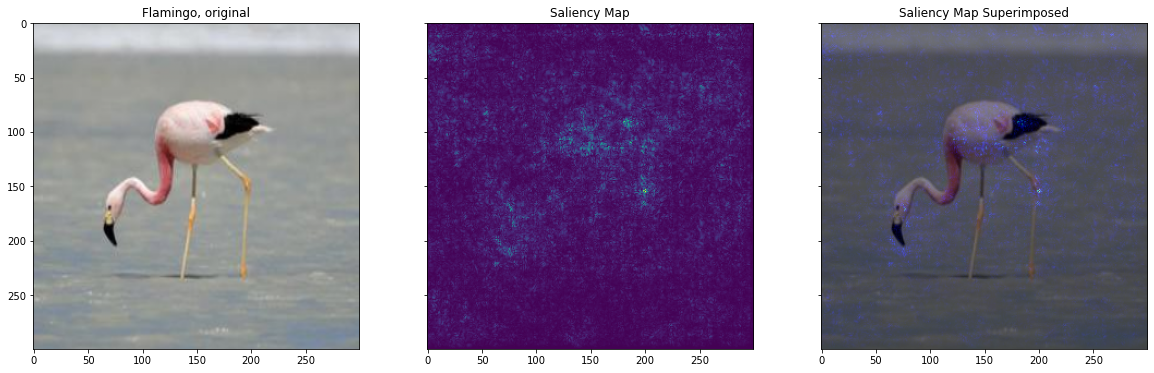
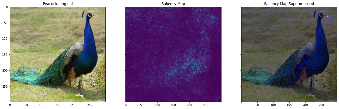
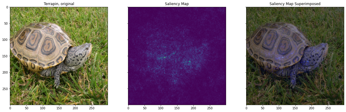
Saliency Maps tells us the parts of the image a model is focusing on… while making its prediction. These are the relevant pixels that can be generated by getting the gradient of the loss wrt the image pixels. i.e the changes in pixels that strongly affect the loss will be shown brightly in our saliency map.

• Acquire the Pretrained Inception Model from Tensorflow Hub
• Preprocess the Images
• Calculate the Gradients
• Create Saliency Map
• Superimpose the map on original image and display

Image Credit: Review of Deep Learning Algorithms for Object Detection

import tensorflow as tf
import tensorflow_hub as hub
import cv2
import numpy as np
import matplotlib.pyplot as plt

Acquire Model

• Acquire the base model from Tensorflow hub
• Append a Softmax activtion
• Build the model based on specified image input shape

model = tf.keras.Sequential([
    hub.KerasLayer('https://tfhub.dev/google/tf2-preview/inception_v3/classification/4'),
    tf.keras.layers.Activation('softmax')
])
model.build([None, 300, 300, 3])

Preprocess

• Read the image
• Convert to RGB colorspace
• Reshape and batch the image

def preprocess(img_file):
    img = cv2.imread(img_file)
    img = cv2.cvtColor(img, cv2.COLOR_BGR2RGB)
    img = cv2.resize(img, (300, 300)) / 255.0

    return img

Calculate Gradients

We want to identify the pixels that are activated for a particular class(for e.g. Peacock, id 84) from the sample picture.

• Set class id of images from imagenet {130: "Flamingo", 84: "Peacock", 36: "Terrapin"}
• Set total number of classes in the training data
• Create an expected output by converting one hot representation to match the final softmax activation layer in the model
• Watch the input pixels through Gradient Tape
• Make predictions and calculate the categorical_crossentropy losses

def calc_gradients(class_idx, preprocessed_image):
    num_classes = 1001
    preprocessed_image = np.expand_dims(preprocessed_image, axis=0)
    expected_output = tf.one_hot([class_idx] * preprocessed_image.shape[0], num_classes)

    with tf.GradientTape() as tape:
        inputs = tf.cast(preprocessed_image, tf.float32)
        tape.watch(inputs)
        predictions = model(inputs)

        loss = tf.keras.losses.categorical_crossentropy(
            expected_output, predictions
        )

    gradients = tape.gradient(loss, inputs)

    return gradients

Create Saliency Map

• Convert the RGB gradient to grayscale
• Normalize the pixel values between the range $[0, 255]$
• Superimpose the saliency map on the original image

def create_saliency_map(gradients):
    grayscale_tensor = tf.reduce_sum(tf.abs(gradients), axis=-1)
    normalized_tensor = tf.cast(
        255
        * (grayscale_tensor - tf.reduce_min(grayscale_tensor))
        / (tf.reduce_max(grayscale_tensor) - tf.reduce_min(grayscale_tensor)),
        tf.uint8,
    )
    normalized_tensor = tf.squeeze(normalized_tensor)

    return normalized_tensor

def superimpose_saliency_map(normalized_tensor, preprocessed_image):
    gradient_color = cv2.applyColorMap(normalized_tensor.numpy(), cv2.COLORMAP_HOT)
    gradient_color = gradient_color / 255.0
    super_imposed = cv2.addWeighted(preprocessed_image, 0.5, gradient_color, 0.5, 0.0)

    return super_imposed

images = {130: "Flamingo", 84: "Peacock", 36: "Terrapin"}
for idx, name in images.items():
    preprocessed_image = preprocess(f"{str(idx)}_{name.lower()}.jpeg")
    gradients = calc_gradients(251, preprocessed_image)
    normalized_tensor = create_saliency_map(gradients)
    super_imposed = superimpose_saliency_map(normalized_tensor, preprocessed_image)

    fig, (ax1, ax2, ax3) = plt.subplots(1, 3, figsize=(20, 6), sharey=True)
    ax1.imshow(preprocessed_image)
    ax2.imshow(normalized_tensor)
    ax3.imshow(super_imposed)
    ax1.set_title(f"{name}, original")
    ax2.set_title(f"Saliency Map")
    ax3.set_title(f"Saliency Map Superimposed")

    plt.show()

Inference

Causality is a deep topic, In this post we introduced causal inferencing and it’s significance over traditional statistical approaches. Further, we explored various schemes of model interpretability. In the final section, using saliency maps we extracted the activated pixels of imagenet classes using inception model and displayed. I planned to go deeper into causal inferencing in the future posts for diverse classification/regression problems.

Reference

• Quantifying Causal Inferences by Janzin et al of Max Planck Institute, 2014
• Causal vs. Statistical Inference by Marin Vlastelica Pogančić, 2019
• Beyond Predictive Models: The Causal Story Behind Hotel Booking Cancellations by Siddharth Dixit, 2020
• Causal Inference: Trying to Understand the Question of Why by Kevin Wang, 2020
• Causal Inference by Lucas et al, 2020
• Introduction to Causal Inference by Brady Neal
• DoWhy – A library for causal inference by Sharma et al of Microsoft, 2018
• Causal Inference: Making the Right Intervention | QuantumBlack by Paul Beaumont, 2019
• Reichenbach’s Common Cause Principle from Stanford Philosopy
• Causality Learning: A New Perspective for Interpretable Machine Learning by Xu et al, 2020
• Causal Interpretability for Machine Learning - Problems, Methods and Evaluation by Moraffah et al ASU, 2020
• Causal Models from Stanford Philosophy
• An Introduction to Causal Inference by Richard Scheines