Bijectors of Tensorflow Probability - A Guide to Understand the Motivation and Mathematical Intuition Behind Them
Posted November 7, 2021 by Gowri Shankar ‐ 11 min read
A bijector is a function of a tensor and its utility is to transform one distribution to another distribution. Bijectors bring determinism to the randomness of a distribution where the distribution by itself is a source of stochasticity. For example, If you want a log density of distribution, we can start with a Gaussian distribution and do log transform using bijector functions. Why do we need such transformations, the real world is full of randomness and probabilistic machine learning establishes a formalism for reasoning under uncertainty. i.e A prediction that outputs a single variable is not sufficient but has to quantify the uncertainty to bring in model confidence. Then to sample complex random variables that get closer to the randomness of nature, we seek the help of bijective functions.
In this post, we shall learn the mathematical intuition and the motivation behind the Bijector functions of Tensorflow in detail, this post is one of many posts that comes under the category Probabilistic Deep Learning focusing on uncertainty and density estimation. Previous posts can be referred to here
Objective
The objective of this post is to understand the bijective functions and their properties to understand the motivation and mathematical intuition behind the Bijectors of Tensorflow Probability(TFP) package.
Introduction
Time travel to your 10th grade - bijections, bijective functions or invertible functions is not something new to us. We have studied them all in our set theory classes, oh yeah they are just maps. Each element of the first set is paired with exactly one set in the second set. The elements of the first set are called the domain and the elements of the second set are called co-domain. Few rules that define what exactly a function is,
- All elements of set 1 must have a pair in the second set
- If set 1 and set 2 elements are related by a single pair then the relationship is called as
one-one function - If more than 1 element in set 1 have the same pair in set 2, then the relationship is called a
many-one function - If every element in set 2 has a corresponding domain and a few elements of set 1 paired to the same element in set 2, then it is called
onto function - surjective, non-injective - If there is an element in the co-domain that has no corresponding domain, then it is called
into function or injective, non-surjective function - If there is at least a single element in set 1 that has no co-domain, then there exists no relationship between set 1 and set 2 - hence that is not a function at all.

That set of rules leaves us with one combination that defines bijection precisely - i.e. A function that is injective, surjective, and one-one is a bijective function, It also means both the sets have the same number of elements. Set theory is cooler than what one can imagine if you closely observe - the whole tech space is built on top of the foundational principles of set theory. A Venn diagram is the classic example of how a relational database works(UNIONS and JOINS) - It is silly to quote yet I am quoting, the term relational in RDBMS is nothing but the above set of rules that we have mentioned to define a function.

Distributions are Sources of Stochasticity
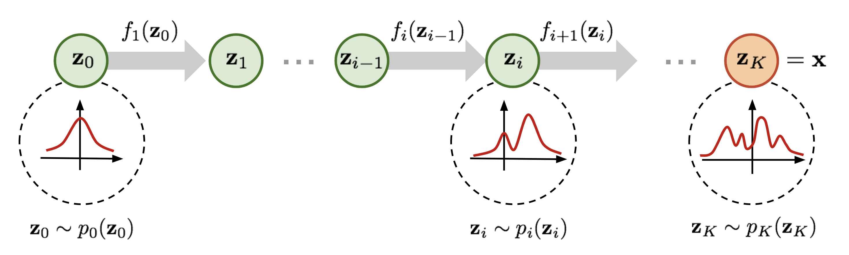
There is too much randomness in nature(pun intended) and we are trying to model these natural phenomenons. It is quite difficult to craft the complex distributions that are resultant of randomness observed from nature, hence we start from something simple, say a Gaussian Distribution. In a Gaussian Distribution, the parameters of interest like mean and standard deviations are constrained but our estimation requires an unconstrained space where a direct sampling is difficult. Traditionally a Markov Chain Monte Carlo method is used for obtaining such sequences of random samples that converge to a target probability distribution, these are time-reversal and volume-preserving in nature. Bijector functions of Tensorflow Probability helps us to create such complex transformation of distributions through a process called Normalizing Flows. Please note, these transformations are deterministic - that is the beauty. Refer to one of our previous articles, a practical guide to normalizing flows to understand implementation details of Bijectors,
The Need for Bijective Functions
In this section, we shall review some of the critical characteristics of Bijective functions - This could be a perfect review of the concepts we often forget when we realize how beguiling math is.
Isomorphism
There are quite a lot of complex definitions for this concept but the one that made me really understand is from graph theory Two graphs G1 and G2 are isomorphic if there exists a matching between their vertices so that two vertices are connected by an edge in G1 if and only if corresponding vertices are connected by an edge in G2. The following diagram makes it much more simple - both these graphs are isomorphic.

- Image Credit: Graph Isomorphisms and Connectivity
The above geometric intuition can be interpreted in many other forms especially via sets but for absolute clarity, we shall study the mathematical intuition through our favorite notations.
Let us have two sets $A$ and $B$ with their corresponding elements ${a_1, a_2, a_3, \cdots, a_n}$ and ${b_1, b_2, b_3, \cdots, b_m}$ respectively, then if there exist a binary mapping $f$ such that
$$\large f(a_i \oplus b_j) = f(a_i) \otimes f(b_j) \tag{1. Isomorphic Mapping}$$ $$\large f^{-1}(b_r \otimes b_s) = f^{-1}(b_r) \oplus f^{-1}(b_s) \tag{2. Inverse Isomorphic Mapping}$$ $$then, \text{they are isomorpmic}$$
From Group theory, isomorphism preserves the structural integrity of a set - It often maps a complicated group to a simpler one.
Homeomorphism - A Donut and A Coffee Mug are Same
How can a donut becomes a coffee mug - by continuous deformation, refer to the animation below. The key point to take from this metaphor is the volume preservation that we have briefly mentioned at the beginning of this post.

- Image Credit: Homeomorphism from Wikipedia
– Wikipedia
The formal definition of homeomorphic function has one-one mapping between sets such that both the function and its inverse are continuous and that in topology exists for geometric figures which can be transformed one into the other by elastic deformation.
Diffeomorphism
If you notice the definition of isomorphism and homeomorphism, the relationship between the sets/groups is established stronger with the addition of more and more properties. This closeness eventually lead to minimal KL-Divergence a common measure of the difference between two distributions or a loss function for stochasticity measurements. A diffeomorphism is a stronger form of equivalence than a homeomorphism. The formal definition of diffeomorphic function is it is a map between manifolds that is differentiable and has a differentiable inverse
More concisely, any object that can be “charted” is a manifold.
One of the goals of topology is to find ways of distinguishing manifolds. For instance, a circle is topologically the same as any closed loop, no matter how different these two manifolds may appear. Similarly, the surface of a coffee mug with a handle is topologically the same as the surface of the donut, and this type of surface is called a (one-handled) torus.
– Wolfram Mathworld
One simple way to understand diffeomorphism is - Let us say we believe ourselves, geometrically speaking a point from nowhere means our beliefs are personal. Then we find another person who has the same beliefs, geometrically a line connecting two points in a 2D space. Similarly, the dimension increases and the belief manifests across through the dimensions. If the beliefs are differentiable and invertible through the dimensions then we call it diffeomorphic bijective belief(function) - pun intended.
Wikipedia says, Given two manifolds ${\displaystyle M}$ and ${\displaystyle N}$, a differentiable map ${\displaystyle f\colon M\rightarrow N}$ is called a diffeomorphism if it is a bijection and its inverse ${\displaystyle f^{-1}\colon N\rightarrow M}$ is differentiable as well. If these functions are ${\displaystyle r}$ times continuously differentiable, ${\displaystyle f}$ is called a ${\displaystyle C^{r}}$-diffeomorphism.
Permutation Group
This is more simple to grasp, the group consisting of all possible permutations of ${\displaystyle N}$ objects is known as the permutation group. of the order ${\displaystyle N}!$
Projective Map
It is all about perspective, imagine a negative film is projected from a distance placed on a plane - that is pixel-pixel, line-line, object-object mapping. Otherwise called isomorphism of vector spaces or tensors. A picture worth a million words also I doubt whether I am qualified enough to scribe this in worlds.

- Image Credit: Homography from Wikipedia
In (1), the width of the side street, W is computed from the known widths of the adjacent shops. In (2), the width of only one shop is needed because a vanishing point, V is visible.
– Wikipedia
Bijectors of Tensorflow Probability
We studied distributions are sources of stochasticity that collects properties of probability that include ${\mu - mean, \sigma - standard deviation}$. Bijectors make the deterministic transformations for the distributions as per the properties and conditions we have studied in the previous sections. They are the abstraction that enables efficient, composable manipulations of probability distributions by ensuring the following,
- Simple but robust and consistent interface for the programmers to manipulate the distributions
- Provide rich high dimensional densities that are invertible and volume-preserving mappings
- Provide efficient and fast volume adjustments through log determinant of the Jacobian matrix concerning dimensionality
- Decouple stochasticity from determinism through simplistic design and flexibility
- Encapsulate the complexities through imparting modularity and exploiting algebraic relationships among random variables
For example, Bijector APIs provides an interface for diffeomorphism for a random variable $\displaystyle X$ and its diffeomorphism $\displaystyle F$ as follows,
$$Y = F(X) \tag{3. Density Function}$$ $$\Large p_{Y(y)} = p_X \left(F^{-1}(y)\right)|DF^{-1}(y)| \tag{4. Diffeomorphism in Bijectors}$$
Where,
- $DF^{-1}$ is the inverse of the Jacobian of $\displaystyle F$
Core of Bijectors
The key objective of a Bijector is to transform a Tensor of certain random distribution to a target distribution and ensure it is invertible. From Joshua V. Dillon et al’s paper title Tensorflow Distributions,
forwardimplements $\displaystyle x \mapsto F(x)$, and is used byTransfromedDistribution.sampletoconvert one random outcome into another. It also establishes the name of the bijector.inverseundeos the transformation $\displaystyle y \mapsto F^{-1}(y)$ and is used byTransfromedDistribution.log_probinverse_log_det_jacobiancomputes $log|DF^{-1}(y)|$ and is used byTransfromedDistribution.log_probto adjust for how the volume changes by the transformation. . In certain settings, it is more numerically stable (or generally preferable) to implement the forward_log_det_jacobian.Because forward and reverse log ◦ det ◦ Jacobians differ only in sign, either (or both) may be implemented.
Conclusion
Probabilistic Machine/Deep Learning gives the measure of uncertainty for our predictions, making it a more human-like approach towards achieving convergence. Although this post is predominantly focused on the properties and mathematical intuition behind bijective functions, the intent is to understand the motivation behind the Bijectors of TFP. I hope I covered all the nuances of bijective functions in detail with relevant examples for the readers’ pleasure. This post is inspired by Joshua V. Dillon et al’s paper on TFP architecture, I thank Joshua and his team for motivating me to write this short one. I also thank my readers and say goodbye until one more adventure with math and its utility.
References
- Isomorphism - Brittanica from Brittanica
- Isomorphic Graphs from Wolfram Mathworld
- Hamiltonian Monte Carlo from Wikipedia
- Bijection from Wikipedia
- Permutation Group from Wolfram Mathworld
- Examples of Homeomorphism in a Sentence from Merriam Webseter
- Diffeomorphism from Wolfram Mathworld
- Diffeomorphism from Wikipedia
- When is a coffee mug a donut? Topology explains it by Mariëtte Le Roux, Marlowe Hood, 2016
- Homography from Wikipedia
- TensorFlow Distributions by Dillon et al of Google, 2017
- Probabilistic Machine Learning in TensorFlow Interview with Joshua Dillon, 2018
– Chris Sutter, 2019