Bayesian and Frequentist Approach to Machine Learning Models
Posted March 27, 2021 by Gowri Shankar ‐ 5 min read
Rev. Thomas Bayes discovered the theorem for conditional probability that bears his name and forms the basis for Bayesian Statistical methods. Sir Ronald Fisher is considered one of the founders of frequentist statistical methods and originally introduced maximum likelihood.
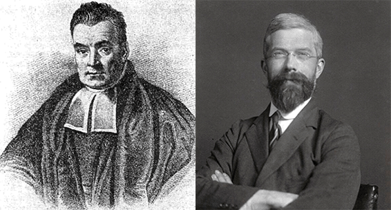
Image Credit: Thomas Bayes and Ronald Fisher
Who are you, a Bayesian or Frequentist?
Introduction
Premisis: Offices are Closed Today, Why?
- Today is Sunday
- Offices are under renovation
- Pandemic days, offices are always closed
- Offices are never opened
Before Covid Days… The most likely argument would be “Offices are closed today” because “Today is Sunday”. That is infered based on 3 principles
- Use
priorknowledge - We know offices arenot neveropened state, that is our prior knowledge. Option 4 is discounted - Explains the most likely observation - We never heard of a pandamic shutdown before, Option 3 has no clear explanation.
- Avoid Unnecessary Assumptions - Renovation by itself requires offices to open for the renovators to get in. Option 2 has an assumption without proof
However, the aberrations caused due to covid pandemic changed our prior knowledge and assumptions significantly to change our priors and beliefs… Hence “Offices are Closed” because “These are Pandemic Days” and the management decided to “Renovate the Property” but “Today is Sunday” hence there are no workers around. That is really chaotic, non linear but beyond any disputes. The new normal is not the normal.
How Frequentist and Bayesians approach a problem?
- Frequentists are Objective and Bayesians are Subjective
- Frequentist believe importance of the features of a dataset is fixed and the observations vary on contrary Bayesians claim feature importance vary but the observations are fixed for example, when you train your model… the observations are fixed and the feature importance vary
- With frequentists approach observations has to be larger than the features, Bayesian approach works for any number of observations
- Frequentists train using maximum likelihood principle, Bayesians compute the posterior using Bayes formula
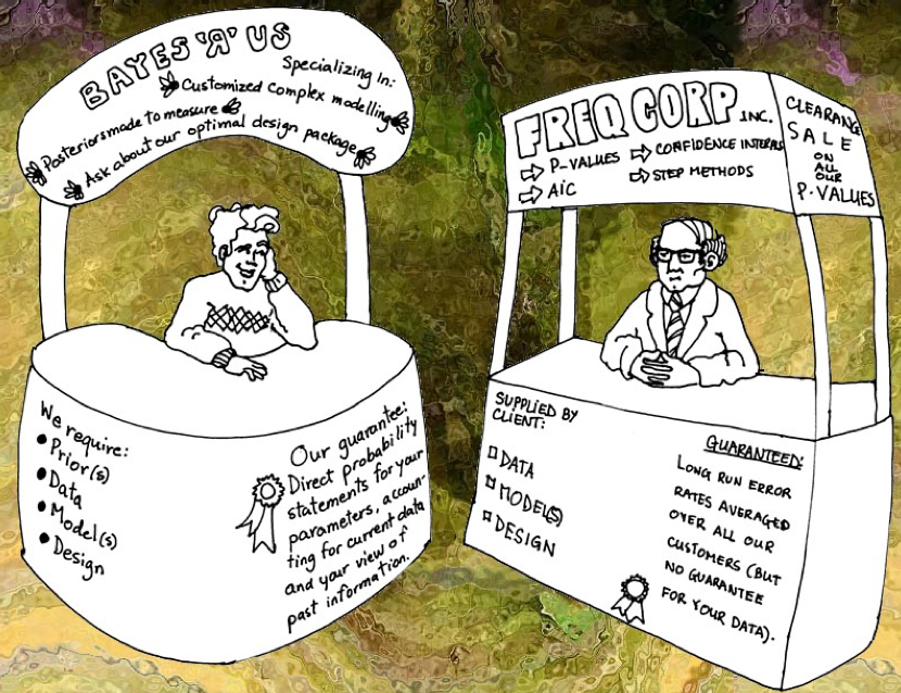 Image Credit: CULTIVATING & CRASHING
Few Details,
What is the probability of someone smokes cigarettes?
A frequentist will say, it is $1/2 = 0.5$
However, A Bayesian seeks information about the person to give a probabilistic answer
What is a feature importance?
For example, a linear model can be defined as follows
$$y = \theta_w x + \theta_b$$
Where, $\theta_w$ is the feature importance for the feature $x$ and the interept(or bias) $\theta_b$ also adds the contribution
What is Maximum Likelihood Principle?
For simplicity, let us assume the data is normally distributed. We have to identify the mean($\mu$) and the standard deviation($\sigma$) responsible for arriving at the dataset. The process involved in finding right mean and standard deviation for a dataset is Maximum Likelihood Estimation. It is defined as
$$\hat\theta = argmax P(X|\theta)$$
ie. a frequentist try to find the features$(\theta)$ that maximize the likelihood$(\hat\theta)$ of the outcome probability.
How to compute posteriors?
The process of identifying the probability of the outcome given the data using Bayes theorem.
$$P(\theta|X) = \frac{P(X|\theta)P(\theta)}{P(X)}$$ ie. For a given prior belief $P(\theta)$ that the obervations $X$ have a likelihood $P(X|\theta)$ with an evidence $P(X)$ posterior is $P(\theta|X)$
$$i.e.$$ $$Posterior = \frac{Likelihood \times Prior} {Evidence}$$
Maximum Likelihood Estimation
Let $X = {x_1, x_2, \cdots, x_N}$ be the observed data for a model with weight $\theta$. Then $P(X|\theta)$ is the likelihood which is a function of a vector of $\theta$s. For simplicity, let us draw samples independently from the normal distribution with unknown parameters which is a function of $(\mu, \sigma)$. Then the probability dennsity for a single observation
$$P(x_i;\mu, \sigma) = \left(\frac{1}{2\pi\sigma^2}\right)^{1/2}exp\left(-\frac{(x_i - \mu)^2}{2\sigma^2}\right)$$ then for N observations, $$P({x_1, x_2, \cdots, x_N}; \mu, \sigma = P(x_1;\mu, \sigma) \times P(x_2;\mu, \sigma) \times P(x_3;\mu, \sigma) \cdots P(x_n;\mu, \sigma)$$ $i.e.$ $$P(X;\mu, \sigma) = \left(\frac{1}{2\pi\sigma^2}\right)^{N/2}exp\left(-\frac{1}{2\sigma^2}\sum_{i=1}^N(x_i - \mu)^2\right)$$ $$\prod_{i=1}^N P(x_i; \mu, \sigma^2)$$
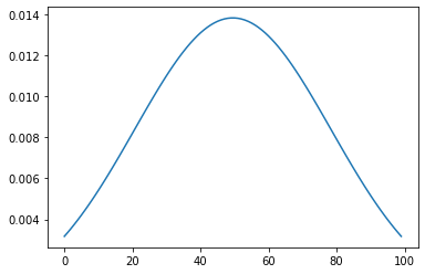
As discussed above, MLE for parameter is the value of $\theta$ that maximizes the likelihood. It is the most common way to estimate unknown variables. Let us write a small peace of code to confirm the same.
import numpy as np
import math
import matplotlib.pyplot as plt

def my_pdf(x_i, mean, std):
    part_1 = np.sqrt(1.0 / (2 * math.pi * std ** 2))
    part_2 = np.exp(- ((x_i - mean) ** 2) / (2 * std ** 2))
    return part_1 * part_2
x = np.arange(100) # Get first hundred numbers and plot the PDF.
mean = np.mean(x)
std = np.std(x)

pdf = []
for an_x in x:
    pdf.append(my_pdf(an_x, mean, std))
plt.plot(x, pdf)
plt.show()
We assumed, the observations are independent and the likelihood take s the form of a product of individual likelihoods for each samples. Let us find the maximum of the function. ie $$log_p(X|\theta) = \sum_{i=1}^N log_p(x_i|\theta)$$ the above equation takes the form of the sum of individual log likelihood functions as follows $$log_p(x_i|\theta) = - \frac {N}{2} log(2\pi\sigma^2) - \frac{1}{2\sigma^2}\sum_{i=1}^N(x_i -\mu)^2$$
Maximizing this expression with respect to $\mu$ $$\frac{\partial}{\partial\mu}p(X; \mu, \sigma) = - \frac{1}{\sigma^2}\sum_{i=1}^N(x_i - \mu) = 0$$
This process is a analytically intractable, but numerica solutions through iterative methods like Expectation Maximization Algorithms estimates well.
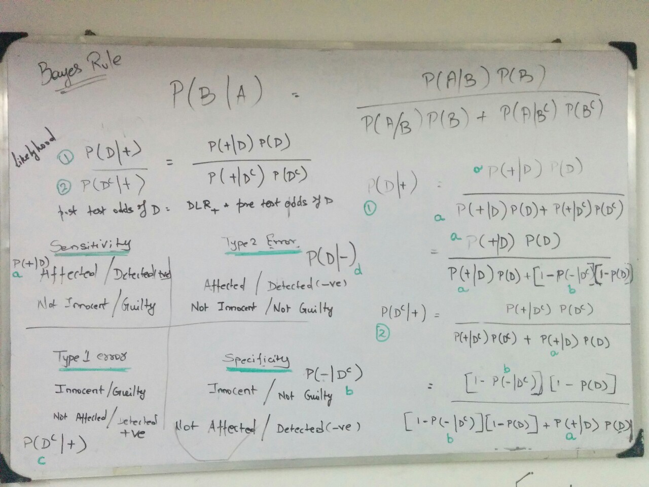
Bayes Theorem
Bayes theorem is simple and powerful to compute the probabilities when there are certain knowns. We know the conditional probability $$P(\theta|X) = \frac{P(\theta \cap X)}{P(X)}$$ $$P(X|\theta) = \frac{P(X \cap \theta)}{P(\theta)}$$
Since $P(\theta \cap X)$ equals $P(X \cap \theta)$, by substitution $$P(\theta|X) = \frac{P(X|\theta)P(\theta)}{P(X)}$$
Let us explain with a concrete example with slightly changed notation in the context testing a patient for a disease Here,
- $D$ Disease detected positive
- $\bar D$ Disease detected negative
- $\oplus$ Patient Sick
- $\ominus$ Patient Not Sick
i.e. $D$ denotes the test result, +/- denotes the patient condition
What is the probability of test results comes +ve and the patient is sick $P(D|\oplus)$?
$$P(D|\oplus) = \frac{P(\oplus|D)P(D)}{P(\oplus|D)P(D) + P(\oplus|\bar D)P(\bar D)}$$ $$i.e.$$ $$P(D|\oplus) = \frac{P(\oplus|D)P(D)}{P(\oplus|D)P(D) + (1 - P(\ominus|\bar D))(1 - P(D))}$$
What is the probability of test results comes -ve and the patient sick $P(\bar D | \oplus)$?
$$P(\bar D|\oplus) = \frac{P(\oplus|\bar D)P(\bar D)}{P(\oplus|\bar D)P(\bar D) + P(\oplus|D)P(D)}$$ $$i.e.$$ $$P(\bar D|\oplus) = \frac{(1 - P(\ominus|\bar D))(1 - P(D))}{(1 - P(\ominus|\bar D))(1 - P(D)) + P(\oplus|D)P(D)}$$
From above equations, given certain probabilities… other unknown probabilities can be computed.
Below table shows the notations for the 4 key parameters that Bayes Theorem unravel.
| * | Test $\oplus$ | Test $\ominus$ |
|---|---|---|
| Sick | Sensitivity $P(\oplus|D)$ | Type 2 Error $P(D|\ominus)$ |
| Not Sick | Type 1 Error $P(\bar D|\oplus)$ | Specificity $P(\ominus|\bar D)$ |
Conclusion
This post gave an insight about how Frequentists and Bayesians think and thier supporting arguments. From this introduction, we shall build Bayesian way of thinking in the future posts.
Years back I tried to fit Bayes Theorem in one board… down memory lane…