Counterfactuals are powerful methodologies of causal reasoning, we introduced causal condition from counterfactuals as a compelling concept to address model explaination, trustworthiness, fairness and out of distribution/domain(OOD) issues in our earlier articles. This is our 3rd post on causality, Please refer…

• Causal Reasoning, Trustworthy Models and Model Explainability using Saliency Maps
• Is Covid Crisis Lead to Prosperity - Causal Inference from a Counterfactual World Using Facebook Prophet

In this post, we shall explore 3 mechanisms of model explanations. They are

• SHAP - SHapley Additive exPlanations
• LIME - Local Interpretable Model-Agnostic Explanations
• DiCE - Diverse Counterfactual Explanations

• Image Credit: The Best of All Possible Worlds

Objectives

Objective of this post is to understand the mathematical intuition behind SHAP, LIME and DiCE.

Introduction

Machine learning models evolved leap and bound over the past few years, they are widely adopted across various industries and domains of business. Despite their popularity, they still remain black boxes which makes them quite unacceptable in areas like healthcare, aviation etc where the stakes are high. Hence, there is a high demand for explanation, interpretation and transparency of the model behavior to deploy AI inspired solutions in mission critical applications. As introduced earlier, model explainability/interpretability mechanisms are broadly classified into 2,

• Attribution based, ranking of the feature vectors and
• Counterfactuals based, explanations provided through counterfactual examples

SHAP and LIME are widely adopted attribution based model explainability mechanisms and DiCE is a counterfactual based causal inferencing scheme. Mothilal et al in their paper titled Towards Unifying Feature Attribution and Counterfactual Explanations: Different Means to the Same End proposed a novel scheme of unifying attribution and counterfactuals through a property called actual causality. Actual causality is empirically calculated using 2 attributes necessity and sufficieny.

Where, necessity is a feature value necessary for generating the model’s output and sufficiency is the feature value sufficient for generating the model output. A unifying framework is an interesting topic to analyze but for a different day. In this post we shall dive deep inside the internals of 3 schemes of interest that we have listed in the opening note.

What could be the ideal scenario, for example a linear model has $n$ number of features $x_1, x_1, x_2, \cdots, x_n$ and their corresponding importance as weight is $w_1, w_2, w_3, \cdots, w_n$ and the predicted outcome is $\hat y$.

$$f(x) = b + w_1 x_1 + w_2 x_2 + \cdots + w_i x_i + \cdots + w_n x_n$$ $$i.e.$$ $$f(x) = \sum_{i=1}^n w_i x_i + b$$

Let us say $\phi_i$ is the contribution of the feature $x_i$ for the predicted outcome $\hat y$, then $$\phi_i(f, x) = w_i x_i - E(w_i X_i) = w_i x_i - w_iE(x_i) \tag{1. Contribution of Single Feature}$$ Where, $E(w_i X_i)$ is the mean effect estimate of feature $i$. Precisely, the contribution of $i^{th}$ feature is the difference between the feature effect and the average effect.

Since we know how to calculate the contribution of a single feature, overall contribution can be calculated by summing the individual contributions. $$\sum_{i=1}^n \phi_i(f, x) = \sum_{i=1}^n (w_i x_i - E(w_i x_i))$$ $$Considering \ the \ intercept \ b$$ $$\sum_{i=1}^n \phi_i(f, x) = (b + \sum_{i=1}^n w_i x_i) - (b + \sum_{i=1}^n E(w_i x_i))$$ $$i.e$$ $$\sum_{i=1}^n \phi_i(f, x) = \hat y - E(\hat y) \tag{2. Overall Contribution}$$

Is this even possible? in real dataset, NO but for a linear model it works well. However, the premises we set through $eqn.2$ will help us to build a model agnostic scheme to identify feature importance.

SHAP - Explanation Through Feature Importance

Among all, SHAP is quite popular and widely adopted scheme for model explanation. SHAP is a cooperative game theory based mechanism uses Shapley value, this mechanism treats each and every feature of the dataset as a gaming agent(player) and quantify efficiency, symmetry, linearity and null player properties empirically. The success of Shapley values is it’s ability to effectively align with human intuition by discriminating the features with their performance indicators.

Estimating Shapley Value

Let us say, we have a set of features$F$ of size $n$ and SHAP method requires retraining the model on all feature subsets $S \subseteq F$. Based on the model’s performance, an importance value for each feature is assigned.

i.e,

• $f_{S \cup {i}}$ is a model, trained having the feature $i$
• $f_S$ is another model, trained without the feature $i$

Then predictions from both the models are compared using a values of input features$(x_S)$ present in the set $S$ as follows

$$f_{S \cup {i}}(X_{S \cup {i}}) - f_S(x_s)$$

Then the Shapley values are computed and used as feature attributions, they are weighted average of all possible differences

$$ \phi_i = \sum_{S \subseteq F \text{ \ } {i}} \frac{|S|!(|F| - |S| - 1)}{|F|!}[f_{S \cup {i}}(X_{S \cup {i}}) - f_S(x_s)] \tag{3. Shapley Estimator}$$

LIME - Explanation through Examples

LIME methodology is built based on inspecting individual predictions and their explanations by aiding users through suggestions of which instances to inspect(It works even for large datasets). Like SHAP, LIME is a model agnostic scheme for any classifier or a regressor. This process of picking and choosing individual predictive models are called as local surrogates. Local surrogate models are constructed by generating new dataset consisting of perturbed samples and then trained. Then the actual dataset is fed to the surrogate model and differences are approximated. This process of perturbation and prediction on original dataset is called as local fidelity.

Fidelity - Interpretability Trade-off

Let us define an explanation for a model $g \in G$ as follows, where $G$ is a class of potentially interpretable models.

• $\Omega (g)$: We introduce a complexity factor $\Omega (g)$, where we cannot easily interpret all the models $g \in G$.
• Let $f$ be the model being explained for a classification problem, $f(x)$ is the probability that $x$ belongs to a certain class $c_1$.
• $\pi_x(z)$: It is the proximity measure between an instance $z$ to $x$, i.e perturbed data surrogate model’s outcomes for actual data

Then, the measure of unfaithfulness of the model g is $$\xi (x) = argmin_{g \in G} \mathcal{L}(f, g, \pi_x) + \Omega(g) \tag{4. Unfaithfulness Measure}$$

DiCE - Counterfactual Generation Engine

Refer here for introduction to counterfactuals and a sample set created with a counterfactual assumption,

• Is Covid Crisis Lead to Prosperity - Causal Inference from a Counterfactual World Using Facebook Prophet

We have a dataset $x$ and we want to create an alternate universe with $n$ counterfactual examples ${c_1, c_2, c_3, \cdots, c_n}$ contradicting the original dataset using a predictive mode $f$ which is static and differentiable. Our goal is to ensure the counterfactual set ${c_1, c_2, c_3, \cdots, c_n}$ is actionable rather than a fiction.

• CF examples generated are to be feasible with original input dataset $x$
• Diversity in generated data to create alternate outcomes
• Measure diversity using a diversity metrics for the counterfactuals
• Ensure feasibility with $x$ using proximity constraints

In the following sections we shall see diversity measures and proximity constraints in detail. Feasibility is beyond the scope of this article, we shall see it in one of the future posts.

Diversity of Counterfactuals

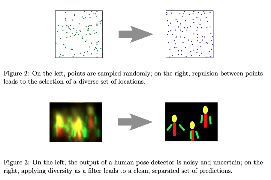
Diversity of counterfactuals are designed using Determinantal Point Process(DPP), an elegant problistic models of repulsion that arise in quantum physics and random matrix theory. DPPs offer efficient and exact algoritms for sampling, marginalization, conditioning and other inferential tasks. Refer Determinantal point processes for machine learning

$$dpp_{diversity} = det(K)$$ $$where$$ $$K_{i,j} = \frac{1}{1 + dist(c_i, c_j)} \tag{5. Diversity}$$ here $dist(c_i, c_j)$ denotes a distance metric between two counterfactual examples.

This image illustrates how DPP applies diversity through repulsion.

• Image Credit: Determinantal point processes for machine learning

Proximity of Counterfactuals

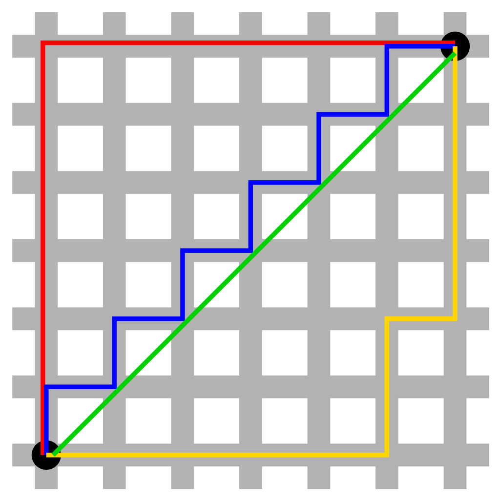
Having higher proximity of a counterfactual to original inputs are ensures easy interpretability. For e.g. flipping the gender, changing the nationality that lead to change in the outcome. Hence, we quantify proximity as the vector distance between original input and CF example’s feature. This is typically a Manhattan distance or L1 norm, which is a distance between two points in a N dimensional vector space.

$$Proximity = - \frac{1}{k} \sum_{i=1}^k dist(c_i, x) \tag{6. Proximity}$$

Manhattan Distance vs Euclidean through Taxicab geometry: In taxicab geometry, the red, yellow, and blue paths all have the same shortest path length of 12. In Euclidean geometry, the green line has length and is the unique shortest path.

• Image Credit: Taxicab geometry

Optimization of CF Generator

Counterfactuals can be generated with trial and error, that we did in our earlier post on Covid Crisis Impact on NFTY50. We had prior knowledge of the event hence the outcomes generated created a sensible counterfactual world. However, our hypothesis is to create CFs based on the following,

• Diversity
• Proximity and
• Feasibility

Since we measure them empirically and they are differentiable, we can define a loss function that combines over diversity and proximity of all generated counterfactuals.

$$\mathcal{C}(x) = argmin_{{c_1, \cdots, c_n}} \frac{1}{n} \sum_{i=1}^n \mathcal{L}(f(c_i), y)$$ $$ + $$ $$\frac{\lambda_1}{n} \sum_{i=1}^n dist(c_i, x)$$ $$ - $$ $$\lambda_2 dpp_{diversity}(c_1, c_2, c_3, \cdots, c_n) \tag{7. Optimization Loss Function}$$

Where,

• $c_i$ is a counterfactual example(CF)
• $n$ is the total nuber fo CFs generated
• $f(.)$ is the Machine Learning model
• $\mathcal{L}(.)$ is a metric that minimizes the distance between prediction for $c_is$ and the desired outcome $y$
• $\lambda_1, \lambda_2$ are hyperparameters that balance the three parts of the loss function

Optimization is implemented through gradient descent, We shall see this in depth in the forthcoming posts.

Inference

In the previous posts, we introduced causality as a concept and in this post we went deeper to understand the mathematical intuition behind cause and effect. We picked three schemes, 2 on attribution based and 1 on counterfactuals. Our goal was to understand the difference between the attribution and counterfactual mechanisms through architecture of SHAP, DiCE and LIME and I believe we achieved the same. In the future posts, I planned to go little more deeper into counterfactual mechanism to understand alternate universe, finally a practical implementation or a guide that helps how to use these schemes on real world datasets.

Reference

• LIME: “Why Should I Trust You?” Explaining the Predictions of Any Classifier Ribieiro et al of University of Washington
• SHAP: A Unified Approach to Interpreting Model Predictions Lundverg et al, NeurIPS, 2017
• DiCE: Explaining Machine Learning Classifiers through Diverse Counterfactual Explanations Mothilal, Sharma et al, Microsoft Research
• Towards Unifying Feature Attribution and Counterfactual Explanations: Different Means to the Same End Mothilal, Sharma et al, Microsoft Research
• Interpretable Machine Learning Christoph Molnar, 2021
• Determinantal point processes for machine learning Kulesza and Taskar, 2013
• DiCE -ML models with counterfactual explanations for the sunk Titanic Yuya Sugano, 2020
• DiCE: Diverse Counterfactual Explanations for Hotel Cancellations by Micahel Grogan, 2020
• Understanding model predictions with LIME Lars Hulstaert, 2018
• Taxicab geometry Wikipedia