Atoms and Bonds - Graph Representation of Molecular Data For Drug Detection
Posted October 2, 2021 by Gowri Shankar ‐ 15 min read
In computer science, a graph is a powerful data structure that embodies connections and relationships between nodes via edges. A graph illustration of information strongly derives its inspiration from nature. We find a graph or graph-like formations everywhere in nature, from bubble foams to crushed papers. E.g. the cracked surfaces of a dry riverbed or a lake-bed during the dry season is a specialized topological design of graph data structure called Gilbert Tesselations. Soap bubbles and foams form double layers that separate the films of water from pockets of air made up of complex forms of curved surfaces, edges, and vertices. They form the bubble clusters and these clusters are represented as Mobius-invariant power diagrams, one another special kind of graph structure. Conventional DL algorithms restrict themselves to the tabular or sequential representation of data and lose their efficacy. However, Message Passing NN architecture(MPNN) is a Graph Neural Network(GNN) scheme where we can input graph information without any transformations. MPNNs are used in the field of drug detection and it inspired we can model molecular structures for penetrating blood-brain barrier membrane.
This is the third post on Graph Neural Networks, earlier we studied the mathematical foundation behind GNNs in brief and developed a node classifier using Graph Convolution Networks. In this post, we understand MPNNs and their significance in accepting undirected graph data as input without any transformations. Previous posts can be referred to here,
- Introduction to Graph Neural Networks
- Graph Convolution Network - A Practical Implementation of Vertex Classifier and it’s Mathematical Basis

- Image Credit: Molecules
Objective
The objective of this post is to understand the mathematical intuition behind Message Passing Neural Networks. In this quest, we shall briefly study few cheminformatics concepts focusing on the data representation of molecular structures and prepare the data for building deep learning models.
We are not building the MPNN Model now, it is for another day
Introduction
The exciting truth about machine learning is its scheme of work is quite close to science and nature because we are trying to model the elements of nature and its phenomenon to see the elegance in it. The idea of GNN is relatively novel to AI/ML fraternity and it enables us to think and admire various use cases having significant proximity with foundational science. Two reasons inspired me to write this post
- Graph theory and GNNs in predicting quantum properties of molecular materials
- Its application in Drug Detection for Blood-Brain Barrier Penetration modeling
Though we are not going deeper into building the model, there is quite a lot of fun in understanding the concepts of Cheminformatics and data representations.
Gilmer et al in their paper titled Neural Message Passing for Quantum Chemistry demonstrated deep learning models for chemical prediction problems by learning features from the molecular graphs directly and are invariant to graph isomorphism
Graph Isomorphism: There are quite a lot of complex definitions for this concept but the one that made me really understand is Two graphs G1 and G2 are isomorphic if there exists a matching between their vertices so that two vertices are connected by an edge in G1 if and only if corresponding vertices are connected by an edge in G2. The following diagram makes it much more simple - both these graphs are isomorphic.

- Image Credit: Graph Isomorphisms and Connectivity
Math Behind MPNN
The molecules of materials can be represented as Graph structures where atoms are the vertices and bonds are the edges. A MPNN architecture takes an undirected graph with node features $x_v$ and bond feature $e_{vw}$ as input. With these features as input, MPNN operates at 2 phases
- Message Passing Phase and
- Readout Phase
In the message-passing phase, information is propagated across the graph to build the neural representation of the graph, and the readout phase is when the predictions are made. Wrt molecular graphs, the goal is to predict the quantum molecular properties based on the topology of the molecular graph.
For each vertex $v$, there is an associated hidden state and their messages at every time step $t$. $$\Large m_v^{t+1} = \sum_{w \in N(v)} M_t(h_v^t, h_w^t, e_{vw}) \tag{1. Messages associated to the vertex }$$ $$\Large h_v^{t+1} = U_t(h_v^t, m_v^{t+1}) \tag{2. Hidden state for the vertex}$$
Where,
- $e_{vw}$ is the edge feature
- $M_t$ is message functions
- $U_t$ is vertex update functions
- $N(v)$ us the neighbors of $v$ in the graph
In the readout phase, a readout function is applied to the final hidden states $h_v^T$ to makes the predictions, $$\Large \hat y = R({h_v^T|v \in G}) \tag{3. Predicted Quantum Properties}$$
Where $G$ is the molecular graph.
It would be possible to learn edge features using an MPNN by introducing hidden states for all edges in the graph $h_{e_{vw}}^t$ and updating them as was done with equations 1 and 2.
Atoms and Bonds
It is imperative, in order to achieve efficiency and efficacy - the proximity of the inputs to our machine learning model should be closer to the representation of information governed by the laws of nature. i.e The tabular form of representing a graph data structure using an adjacency matrix is good but not great. Hence we seek few novel approaches to create the feature vectors.
In this section, we shall load the Blood-Brain Barrier dataset with ~2000 molecules represented as a human-readable string and craft a graph representation with its feature vectors.
import tensorflow as tf
import pandas as pd
file_path = tf.keras.utils.get_file(
    "BBBP.csv", "https://deepchemdata.s3-us-west-1.amazonaws.com/datasets/BBBP.csv"
)
df_bbbp = pd.read_csv(file_path)
df_bbbp.head()
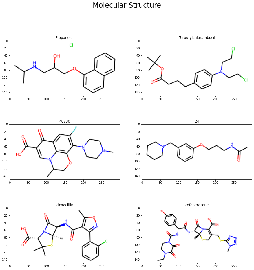
| num | name | p_np | smiles | |
|---|---|---|---|---|
| 0 | 1 | Propanolol | 1 | [Cl].CC(C)NCC(O)COc1cccc2ccccc12 |
| 1 | 2 | Terbutylchlorambucil | 1 | C(=O)(OC(C)(C)C)CCCc1ccc(cc1)N(CCCl)CCCl |
| 2 | 3 | 40730 | 1 | c12c3c(N4CCN(C)CC4)c(F)cc1c(c(C(O)=O)cn2C(C)CO... |
| 3 | 4 | 24 | 1 | C1CCN(CC1)Cc1cccc(c1)OCCCNC(=O)C |
| 4 | 5 | cloxacillin | 1 | Cc1onc(c2ccccc2Cl)c1C(=O)N[C@H]3[C@H]4SC(C)(C)... |
SMILES: SMILES $\rightarrow$ Simplified Molecular-Input Line-Entry System, a scheme for describing the structure of chemical substances or chemically identified molecules using short ASCII strings. SMILES strings are standardized formats with the extensive backing of graph theory through which we can convert the molecular structure into 2-D or 3-D drawings.
SMILES Data
Our first step is to convert the smiles data into a graph representation, this is done with two process
- SMILES to molecule using a cheminformatics package called RDKit
- Graph from molecules
We shall read the smile data and draw the graph using the RDKit library
from rdkit import Chem, RDLogger
import matplotlib.pyplot as plt
import numpy as np
choices = np.random.choice(len(df_bbbp), 6)
molecules = []
for index in np.arange(6):
    row = df_bbbp.iloc[index]
    m = Chem.MolFromSmiles(row["smiles"], sanitize=False)
    molecules.append({"m": m, "name": row["name"]})
molecules
[{'m': <rdkit.Chem.rdchem.Mol at 0x7fd7f8d55580>, 'name': 'Propanolol'},
 {'m': <rdkit.Chem.rdchem.Mol at 0x7fd7f8d6cee0>,
  'name': 'Terbutylchlorambucil'},
 {'m': <rdkit.Chem.rdchem.Mol at 0x7fd7f8d6cf30>, 'name': '40730'},
 {'m': <rdkit.Chem.rdchem.Mol at 0x7fd7f8d6cf80>, 'name': '24'},
 {'m': <rdkit.Chem.rdchem.Mol at 0x7fd7f8d6cdf0>, 'name': 'cloxacillin'},
 {'m': <rdkit.Chem.rdchem.Mol at 0x7fd7f8d6ce90>, 'name': 'cefoperazone'}]
fig, axs = plt.subplots(3, 2, figsize=(15, 15))
fig.suptitle(f"Molecular Structure", size=24)
row = 0
col = 0

for index in np.arange(len(molecules)):
    img = Chem.Draw.MolToImage(molecules[index]["m"], size=(300, 150), kekulize=True, wedgeBonds=True)
    axs[row, col].imshow(img)
    axs[row, col].set_title(molecules[index]["name"])
    col += 1

    if(col == 2):
        row += 1
        col = 0
Features of a Chemical Component
To do effective feature engineering, we have to have a microscopic view of the elements of the molecules - atoms and bonds. A chemical substance is nothing but the culmination of the atomic elements and their relationship with neighbor elements through bonds. Following are the properties of an Atom - i.e. Vertex properties $x_v$
- Symbol, Every atom in the periodic table is represented with a symbol - For e.g $C \rightarrow Carbon$, $Na \rightarrow Sodium$, $H \rightarrow Hydrogen$
- Valence Electron Count, Valence electron is the number of electrons in the outermost orbit of an atom. These electrons participate in the formation of a chemical bond
- Hydrogen Atom Count, Hydrogen atom with a single electron is the lightest element that can readily form a covalent bond, critical for the formation of the molecular structure and function.
- Orbital Hybridization, the phenomenon of mixing atomic orbitals to form new hybrid orbitals suitable for the pairing of electrons to form chemical bonds.
{
    "symbol": {"B", "Br", "C", "Ca", "Cl", "F", "H", "I", "N", "Na", "O", "P", "S"},
    "n_valence": {0, 1, 2, 3, 4, 5, 6},
    "n_hydrogens": {0, 1, 2, 3, 4},
    "hybridization": {"s", "sp", "sp2", "sp3"},
}
Along with the properties of the atoms, we add the properties of the bonds - These are the edge properties $e_{vw}$
- Bond Type, Four types of bonds can occur - Single, Double, Triple, and Aromatic bonds
- Conjugated Systems, It is a system of connected p-orbitals with delocalized electrons in a molecule.
{
    "bond_type": {"single", "double", "triple", "aromatic"},
    "conjugated": {True, False},
}
Atomic Orbital. In quantum mechanics, an atomic orbital or p-orbital is a mathematical function describing the location and wave-like behavior of an electron in an atom.
Delocalized Electrons. Delocalized electrons are electrons in a molecule, ion, and solid metal that are not associated with a single atom or a covalent bond.
I have created a utility python file having the Atom and Bond feature module and SMILES to Graph Conversion module developed by Alexander Kensert. Please refer his work here
Graphs from SMILES
Graph construction of molecular structures are done from SMILES data using the following utilities
- Atom Featurizer
- Bond Featurizer
- SMILES to Molecule Converter
- Molecules to Graph Converter to create atom feature vector, bond feature vector and their pair indices.
from featurizer import AtomFeaturizer, BondFeaturizer
atom_featurizer = AtomFeaturizer(
    allowable_sets={
        "symbol": {"B", "Br", "C", "Ca", "Cl", "F", "H", "I", "N", "Na", "O", "P", "S"},
        "n_valence": {0, 1, 2, 3, 4, 5, 6},
        "n_hydrogens": {0, 1, 2, 3, 4},
        "hybridization": {"s", "sp", "sp2", "sp3"},
    }
)

bond_featurizer = BondFeaturizer(
    allowable_sets={
        "bond_type": {"single", "double", "triple", "aromatic"},
        "conjugated": {True, False},
    }
)
from smiles import graphs_from_smiles, molecule_from_smiles
graph_data = graphs_from_smiles(df_bbbp.smiles, atom_featurizer, bond_featurizer)
RDKit ERROR: [17:16:27] Explicit valence for atom # 1 N, 4, is greater than permitted
RDKit ERROR: [17:16:27] Explicit valence for atom # 6 N, 4, is greater than permitted
RDKit ERROR: [17:16:27] Explicit valence for atom # 6 N, 4, is greater than permitted
RDKit ERROR: [17:16:28] Explicit valence for atom # 11 N, 4, is greater than permitted
RDKit ERROR: [17:16:28] Explicit valence for atom # 12 N, 4, is greater than permitted
RDKit ERROR: [17:16:28] Explicit valence for atom # 5 N, 4, is greater than permitted
RDKit ERROR: [17:16:28] Explicit valence for atom # 5 N, 4, is greater than permitted
RDKit ERROR: [17:16:28] Explicit valence for atom # 5 N, 4, is greater than permitted
RDKit ERROR: [17:16:28] Explicit valence for atom # 5 N, 4, is greater than permitted
RDKit ERROR: [17:16:28] Explicit valence for atom # 5 N, 4, is greater than permitted
RDKit ERROR: [17:16:28] Explicit valence for atom # 5 N, 4, is greater than permitted
atom_feature, bond_feature, pair_indices = graph_data
atom_feature[0]
<tf.RaggedTensor [[0.0, 0.0, 0.0, 0.0, 1.0, 0.0, 0.0, 0.0, 0.0, 0.0, 0.0, 0.0, 0.0, 1.0, 0.0, 0.0, 0.0, 0.0, 0.0, 0.0, 1.0, 0.0, 0.0, 0.0, 0.0, 0.0, 0.0, 0.0, 1.0], [0.0, 0.0, 1.0, 0.0, 0.0, 0.0, 0.0, 0.0, 0.0, 0.0, 0.0, 0.0, 0.0, 0.0, 0.0, 0.0, 0.0, 1.0, 0.0, 0.0, 0.0, 0.0, 0.0, 1.0, 0.0, 0.0, 0.0, 0.0, 1.0], [0.0, 0.0, 1.0, 0.0, 0.0, 0.0, 0.0, 0.0, 0.0, 0.0, 0.0, 0.0, 0.0, 0.0, 0.0, 0.0, 0.0, 1.0, 0.0, 0.0, 0.0, 1.0, 0.0, 0.0, 0.0, 0.0, 0.0, 0.0, 1.0], [0.0, 0.0, 1.0, 0.0, 0.0, 0.0, 0.0, 0.0, 0.0, 0.0, 0.0, 0.0, 0.0, 0.0, 0.0, 0.0, 0.0, 1.0, 0.0, 0.0, 0.0, 0.0, 0.0, 1.0, 0.0, 0.0, 0.0, 0.0, 1.0], [0.0, 0.0, 0.0, 0.0, 0.0, 0.0, 0.0, 0.0, 1.0, 0.0, 0.0, 0.0, 0.0, 0.0, 0.0, 0.0, 1.0, 0.0, 0.0, 0.0, 0.0, 1.0, 0.0, 0.0, 0.0, 0.0, 0.0, 0.0, 1.0], [0.0, 0.0, 1.0, 0.0, 0.0, 0.0, 0.0, 0.0, 0.0, 0.0, 0.0, 0.0, 0.0, 0.0, 0.0, 0.0, 0.0, 1.0, 0.0, 0.0, 0.0, 0.0, 1.0, 0.0, 0.0, 0.0, 0.0, 0.0, 1.0], [0.0, 0.0, 1.0, 0.0, 0.0, 0.0, 0.0, 0.0, 0.0, 0.0, 0.0, 0.0, 0.0, 0.0, 0.0, 0.0, 0.0, 1.0, 0.0, 0.0, 0.0, 1.0, 0.0, 0.0, 0.0, 0.0, 0.0, 0.0, 1.0], [0.0, 0.0, 0.0, 0.0, 0.0, 0.0, 0.0, 0.0, 0.0, 0.0, 1.0, 0.0, 0.0, 0.0, 0.0, 1.0, 0.0, 0.0, 0.0, 0.0, 0.0, 1.0, 0.0, 0.0, 0.0, 0.0, 0.0, 0.0, 1.0], [0.0, 0.0, 1.0, 0.0, 0.0, 0.0, 0.0, 0.0, 0.0, 0.0, 0.0, 0.0, 0.0, 0.0, 0.0, 0.0, 0.0, 1.0, 0.0, 0.0, 0.0, 0.0, 1.0, 0.0, 0.0, 0.0, 0.0, 0.0, 1.0], [0.0, 0.0, 0.0, 0.0, 0.0, 0.0, 0.0, 0.0, 0.0, 0.0, 1.0, 0.0, 0.0, 0.0, 0.0, 1.0, 0.0, 0.0, 0.0, 0.0, 1.0, 0.0, 0.0, 0.0, 0.0, 0.0, 0.0, 1.0, 0.0], [0.0, 0.0, 1.0, 0.0, 0.0, 0.0, 0.0, 0.0, 0.0, 0.0, 0.0, 0.0, 0.0, 0.0, 0.0, 0.0, 0.0, 1.0, 0.0, 0.0, 1.0, 0.0, 0.0, 0.0, 0.0, 0.0, 0.0, 1.0, 0.0], [0.0, 0.0, 1.0, 0.0, 0.0, 0.0, 0.0, 0.0, 0.0, 0.0, 0.0, 0.0, 0.0, 0.0, 0.0, 0.0, 0.0, 1.0, 0.0, 0.0, 0.0, 1.0, 0.0, 0.0, 0.0, 0.0, 0.0, 1.0, 0.0], [0.0, 0.0, 1.0, 0.0, 0.0, 0.0, 0.0, 0.0, 0.0, 0.0, 0.0, 0.0, 0.0, 0.0, 0.0, 0.0, 0.0, 1.0, 0.0, 0.0, 0.0, 1.0, 0.0, 0.0, 0.0, 0.0, 0.0, 1.0, 0.0], [0.0, 0.0, 1.0, 0.0, 0.0, 0.0, 0.0, 0.0, 0.0, 0.0, 0.0, 0.0, 0.0, 0.0, 0.0, 0.0, 0.0, 1.0, 0.0, 0.0, 0.0, 1.0, 0.0, 0.0, 0.0, 0.0, 0.0, 1.0, 0.0], [0.0, 0.0, 1.0, 0.0, 0.0, 0.0, 0.0, 0.0, 0.0, 0.0, 0.0, 0.0, 0.0, 0.0, 0.0, 0.0, 0.0, 1.0, 0.0, 0.0, 1.0, 0.0, 0.0, 0.0, 0.0, 0.0, 0.0, 1.0, 0.0], [0.0, 0.0, 1.0, 0.0, 0.0, 0.0, 0.0, 0.0, 0.0, 0.0, 0.0, 0.0, 0.0, 0.0, 0.0, 0.0, 0.0, 1.0, 0.0, 0.0, 0.0, 1.0, 0.0, 0.0, 0.0, 0.0, 0.0, 1.0, 0.0], [0.0, 0.0, 1.0, 0.0, 0.0, 0.0, 0.0, 0.0, 0.0, 0.0, 0.0, 0.0, 0.0, 0.0, 0.0, 0.0, 0.0, 1.0, 0.0, 0.0, 0.0, 1.0, 0.0, 0.0, 0.0, 0.0, 0.0, 1.0, 0.0], [0.0, 0.0, 1.0, 0.0, 0.0, 0.0, 0.0, 0.0, 0.0, 0.0, 0.0, 0.0, 0.0, 0.0, 0.0, 0.0, 0.0, 1.0, 0.0, 0.0, 0.0, 1.0, 0.0, 0.0, 0.0, 0.0, 0.0, 1.0, 0.0], [0.0, 0.0, 1.0, 0.0, 0.0, 0.0, 0.0, 0.0, 0.0, 0.0, 0.0, 0.0, 0.0, 0.0, 0.0, 0.0, 0.0, 1.0, 0.0, 0.0, 0.0, 1.0, 0.0, 0.0, 0.0, 0.0, 0.0, 1.0, 0.0], [0.0, 0.0, 1.0, 0.0, 0.0, 0.0, 0.0, 0.0, 0.0, 0.0, 0.0, 0.0, 0.0, 0.0, 0.0, 0.0, 0.0, 1.0, 0.0, 0.0, 1.0, 0.0, 0.0, 0.0, 0.0, 0.0, 0.0, 1.0, 0.0]]>
bond_feature[0]
<tf.RaggedTensor [[0.0, 0.0, 0.0, 0.0, 0.0, 0.0, 1.0], [0.0, 0.0, 0.0, 0.0, 0.0, 0.0, 1.0], [0.0, 0.0, 1.0, 0.0, 1.0, 0.0, 0.0], [0.0, 0.0, 0.0, 0.0, 0.0, 0.0, 1.0], [0.0, 0.0, 1.0, 0.0, 1.0, 0.0, 0.0], [0.0, 0.0, 1.0, 0.0, 1.0, 0.0, 0.0], [0.0, 0.0, 1.0, 0.0, 1.0, 0.0, 0.0], [0.0, 0.0, 0.0, 0.0, 0.0, 0.0, 1.0], [0.0, 0.0, 1.0, 0.0, 1.0, 0.0, 0.0], [0.0, 0.0, 0.0, 0.0, 0.0, 0.0, 1.0], [0.0, 0.0, 1.0, 0.0, 1.0, 0.0, 0.0], [0.0, 0.0, 1.0, 0.0, 1.0, 0.0, 0.0], [0.0, 0.0, 0.0, 0.0, 0.0, 0.0, 1.0], [0.0, 0.0, 1.0, 0.0, 1.0, 0.0, 0.0], [0.0, 0.0, 1.0, 0.0, 1.0, 0.0, 0.0], [0.0, 0.0, 0.0, 0.0, 0.0, 0.0, 1.0], [0.0, 0.0, 1.0, 0.0, 1.0, 0.0, 0.0], [0.0, 0.0, 1.0, 0.0, 1.0, 0.0, 0.0], [0.0, 0.0, 1.0, 0.0, 1.0, 0.0, 0.0], [0.0, 0.0, 0.0, 0.0, 0.0, 0.0, 1.0], [0.0, 0.0, 1.0, 0.0, 1.0, 0.0, 0.0], [0.0, 0.0, 0.0, 0.0, 0.0, 0.0, 1.0], [0.0, 0.0, 1.0, 0.0, 1.0, 0.0, 0.0], [0.0, 0.0, 1.0, 0.0, 1.0, 0.0, 0.0], [0.0, 0.0, 0.0, 0.0, 0.0, 0.0, 1.0], [0.0, 0.0, 1.0, 0.0, 1.0, 0.0, 0.0], [0.0, 0.0, 1.0, 0.0, 0.0, 1.0, 0.0], [0.0, 0.0, 0.0, 0.0, 0.0, 0.0, 1.0], [0.0, 0.0, 1.0, 0.0, 0.0, 1.0, 0.0], [1.0, 0.0, 0.0, 0.0, 0.0, 1.0, 0.0], [1.0, 0.0, 0.0, 0.0, 0.0, 1.0, 0.0], [0.0, 0.0, 0.0, 0.0, 0.0, 0.0, 1.0], [1.0, 0.0, 0.0, 0.0, 0.0, 1.0, 0.0], [1.0, 0.0, 0.0, 0.0, 0.0, 1.0, 0.0], [0.0, 0.0, 0.0, 0.0, 0.0, 0.0, 1.0], [1.0, 0.0, 0.0, 0.0, 0.0, 1.0, 0.0], [1.0, 0.0, 0.0, 0.0, 0.0, 1.0, 0.0], [0.0, 0.0, 0.0, 0.0, 0.0, 0.0, 1.0], [1.0, 0.0, 0.0, 0.0, 0.0, 1.0, 0.0], [1.0, 0.0, 0.0, 0.0, 0.0, 1.0, 0.0], [0.0, 0.0, 0.0, 0.0, 0.0, 0.0, 1.0], [1.0, 0.0, 0.0, 0.0, 0.0, 1.0, 0.0], [1.0, 0.0, 0.0, 0.0, 0.0, 1.0, 0.0], [1.0, 0.0, 0.0, 0.0, 0.0, 1.0, 0.0], [0.0, 0.0, 0.0, 0.0, 0.0, 0.0, 1.0], [1.0, 0.0, 0.0, 0.0, 0.0, 1.0, 0.0], [1.0, 0.0, 0.0, 0.0, 0.0, 1.0, 0.0], [0.0, 0.0, 0.0, 0.0, 0.0, 0.0, 1.0], [1.0, 0.0, 0.0, 0.0, 0.0, 1.0, 0.0], [1.0, 0.0, 0.0, 0.0, 0.0, 1.0, 0.0], [0.0, 0.0, 0.0, 0.0, 0.0, 0.0, 1.0], [1.0, 0.0, 0.0, 0.0, 0.0, 1.0, 0.0], [1.0, 0.0, 0.0, 0.0, 0.0, 1.0, 0.0], [0.0, 0.0, 0.0, 0.0, 0.0, 0.0, 1.0], [1.0, 0.0, 0.0, 0.0, 0.0, 1.0, 0.0], [1.0, 0.0, 0.0, 0.0, 0.0, 1.0, 0.0], [0.0, 0.0, 0.0, 0.0, 0.0, 0.0, 1.0], [1.0, 0.0, 0.0, 0.0, 0.0, 1.0, 0.0], [1.0, 0.0, 0.0, 0.0, 0.0, 1.0, 0.0], [1.0, 0.0, 0.0, 0.0, 0.0, 1.0, 0.0]]>
pair_indices[0]
<tf.RaggedTensor [[0, 0], [1, 1], [1, 2], [2, 2], [2, 1], [2, 3], [2, 4], [3, 3], [3, 2], [4, 4], [4, 2], [4, 5], [5, 5], [5, 4], [5, 6], [6, 6], [6, 5], [6, 7], [6, 8], [7, 7], [7, 6], [8, 8], [8, 6], [8, 9], [9, 9], [9, 8], [9, 10], [10, 10], [10, 9], [10, 11], [10, 19], [11, 11], [11, 10], [11, 12], [12, 12], [12, 11], [12, 13], [13, 13], [13, 12], [13, 14], [14, 14], [14, 13], [14, 15], [14, 19], [15, 15], [15, 14], [15, 16], [16, 16], [16, 15], [16, 17], [17, 17], [17, 16], [17, 18], [18, 18], [18, 17], [18, 19], [19, 19], [19, 18], [19, 10], [19, 14]]>
Inference
This one is not yet another post on graph neural networks, the significant aspect of neural message passing architecture for quantum chemistry is its novel representation of data in the graphical form. The undirected graph data with molecular properties, bond properties, and pair information can be directly fed into a machine learning model without transformation. In this first post on MPNN, we studied the following,
- The objective of MPNN architecture
- Mathematical intuition behind message passing neural networks
- SMILES dataset and its properties
- Visualized the molecular structure and bonds
- Properties of a molecular structure and in-silico representation of them and
- finally, converted SMILES dataset into atoms, bonds, and pair information for a DL model to understand.
In the future posts, we shall examine few other use cases, variants of MPNNs and eventually implement a robust model to detect graph properties. Until then, adios amigos!
References
- Graphs in Nature by David Eppstein, UCI - 2019
- Neural Message Passing for Quantum Chemistry by Gilmer et al from Google Brain and DeepMind, 2017
- A Bayesian Approach to in Silico Blood-Brain Barrier Penetration Modeling by Martins et al, 2012
- Introduction to Message Passing Neural Networks by Kacper Kubara, 2020
- A Graph Theory approach to assess nature’s contribution to people at a global scale by Juan et al, Nature 2021
- Gilbert tessellation from Wikipedia
- Graph Isomorphism from UPenn
- Simplified molecular-input line-entry system from Wikipedia
- Orbital hybridisation from Wikipedia
- Message-passing neural network for molecular property prediction by Alexander Kensert, 2021
- MoleculeNet: A Benchmark for Molecular Machine Learning by Wu et al
- Message Passing Neural Networks for Molecular Property Prediction by Kyle Swanson, MIT, 2019
- MoleculeNet: A Benchmark for Molecular Machine Learning by Wu et al, Stanford, 2018
- Chemical Molecule Drawing with rdkit from Pyth 4 Oceanographers, 2013
– Gilmer, Dahl et al, Google Brain and DeepMind