3rd Wave in India, Covid Debacle Continues - Let us Use Covid Data to Learn Piecewise LR and Exponential Curve Fitting
Posted January 7, 2022 by Gowri Shankar ‐ 8 min read
Deep neural networks models are dominant in their job compared to any other algorithms like support vectors machines or statistical models that are celebrated once. When it comes to big data, without a doubt deep learning models are the defacto choice for convergence. I often wonder what must be making them so efficient, something should be quite obvious and provable. Activation functions, we know activation functions bring in non-linearity to the network layers through the neurons and they do the magic in vogue. ReLU, Sigmoid, and their sister-in-law gang are the piecewise linear functions that create non-linearity to the outcomes. i.e. the activation functions help the neural networks to slice and dice the input space into finer grains and form locally sensitive hash tables. A piecewise linear function in the network can be visualized as a polyhedron(or a cell) with sharp edges is the fundamental building block for achieving convergence in DNNs.
The above explanation for the success of neural networks is most convincing and thought-provoking. Certain beliefs are known, accepted but often unconvincingly because of the gap in understanding the fundamental ideas and concepts. When we attempt to ask more and more questions, we see the light - that is the process of learning. This post has 2 parts, we shall study Piecewise Linear Regression models in the first part and how to fit an exponential curve in the second one. This post falls under the section Fundamentals of AI/ML and Convergence under Math for AI/ML, previous posts under these topics can be referred to here,

I thank Tim Scarfe and fearsome(with his knowledge) Dr. Keith Duggar(MIT PhD) for brilliantly explaining the concept of Activation Functions within the context of Piecewise Linear Functions in their 2022 premiere of machine learning street talk. Without the inspiration from them, this article wouldn’t have been possible.
061: Interpolation, Extrapolation, and Linearisation (Prof. Yann LeCun, Dr. Randall Balestriero)
trivia 1: I just finished watching the first 50 minutes of the MLST latest edition, It was like watching a thriller movie - deeply indebted to Tim, Yannic, and Keith for extraordinary rendition of their craft.
trivia 2: Why we all address Dr.Keith Duggar as Dr.Keith Duggar but his compadre Dr.Tim Scarfe and Dr.Yannic Kilcher as Tim and Yannic is quite beyond the scope of this post
DISCLAIMER: This post is purely for academic purposes. I am not suggesting anything beyond learning goals, the analysis is conducted using the latest Covid-19 data.
Objective
The objective of this post is to understand the Piecewise Linear Regression without much mathematics but through coding. We also study how to fit an exponential curve in the second section. With that quest, we cover the following,
- An explorative analysis of the Covid-19 dataset
- Univariate spline smoothing using SciKit interpolate
- PWLF: Piecewise Linear Fitting library for Piecewise Linear Regression
- Math behind logarithmic fitting
Introduction
We are in the nascent stages of understanding how deep neural network models are bringing accurate predictions. Most of the models are not explainable and lack sufficient trust for the end-user to let the machines make the decisions. Hence, we seek models to provide recommendations with uncertainty measurements to increase their reliability. For example, the right way to find the area under a curve is to look at the curve with a magnifying lens and dissect them using a knife to make smaller rectangles and then sum the area of smaller rectangles. i.e. Divide and Conquer. The same principle is apt for fitting curves. To demonstrate this, let us load the global Covid-19 dataset and then analyze a portion of it.
Covid data used in this analysis is taken from Our World In Date: Coronavirus (COVID-19) Cases on $7^{th}$ Jan 2022, 12 PM IST
import pandas as pd
import numpy as np
import matplotlib.pyplot as plt
import seaborn as sns

#%matplotlib inline
covid_df = pd.read_csv("./owid-covid-data.csv", sep=",", parse_dates=["date"])
print(f"No of features: {covid_df.shape[1]}, No of observations: {covid_df.shape[0]}")
print(f"Start Date: {min(covid_df.date)}, End Date: {max(covid_df.date)}")
No of features: 67, No of observations: 152691
Start Date: 2020-01-01 00:00:00, End Date: 2022-01-06 00:00:00
covid_ind_df = covid_df[covid_df.location == "India"]
covid_ind_df.iloc[:, 0:10].tail()
| iso_code | continent | location | date | total_cases | new_cases | new_cases_smoothed | total_deaths | new_deaths | new_deaths_smoothed | |
|---|---|---|---|---|---|---|---|---|---|---|
| 64766 | IND | Asia | India | 2022-01-02 | 34922882.0 | 33750.0 | 18507.000 | 481893.0 | 123.0 | 270.857 |
| 64767 | IND | Asia | India | 2022-01-03 | 34960261.0 | 37379.0 | 22938.571 | 482017.0 | 124.0 | 246.714 |
| 64768 | IND | Asia | India | 2022-01-04 | 35018358.0 | 58097.0 | 29924.571 | 482551.0 | 534.0 | 279.857 |
| 64769 | IND | Asia | India | 2022-01-05 | 35109286.0 | 90928.0 | 41035.143 | 482876.0 | 325.0 | 288.000 |
| 64770 | IND | Asia | India | 2022-01-06 | 35109286.0 | NaN | NaN | 482876.0 | NaN | NaN |
Covid Diagnosis and Growth Curves
Our goal is to fit the new covid cases(Diagnosis) and the total number of covid cases(Growth) curves under a constrained environment to understand Piecewise Linear Regression. We also fit a Logarithmic curve on the growth curve focusing on the period where the first wave ends and up to the peak of the second wave. Waves often result in exponential growth, hence we choose a logarithmic fitting scheme.
def plot_daily_cases(data, scatter=False, predictions_daily=[], predictions_total=[], titleA="", titleB="", sup_title=""):
fig, axes = plt.subplots(1, 2, figsize=(25, 6))
if(scatter):
axes[0].scatter(data.date.values, data.new_cases.values, label='Observed')
axes[1].scatter(data.date.values, data.total_cases.values, label='Observed')
else:
axes[0].plot(data.date.values, data.new_cases.values, label='Observed')
axes[1].plot(data.date.values, data.total_cases.values, label='Observed')
if(len(predictions_daily) == len(data)):
axes[0].plot(data.date.values, predictions_daily, color="red", linestyle='dashed',
linewidth=5, label='Predicted')
if(len(predictions_total) == len(data)):
axes[1].plot(data.date.values, predictions_total, color="red", linestyle='dashed',
linewidth=5, label='Predicted')
axes[0].legend()
axes[1].legend()
axes[0].set_title(titleA)
axes[1].set_title(titleB)
fig.suptitle(sup_title, fontsize=20)
plt.show()
from scipy.interpolate import UnivariateSpline
def smooth_spline(data, sm_factor=0.5):
spl = UnivariateSpline(np.arange(len(data)), data, s=len(data))
spl.set_smoothing_factor(sm_factor)
return spl(data)
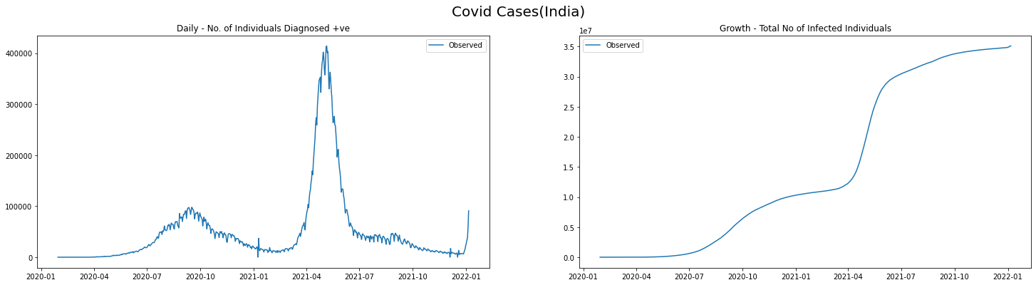
plot_daily_cases(
covid_ind_df,
titleA="Daily - No. of Individuals Diagnosed +ve",
titleB="Growth - Total No of Infected Individuals",
sup_title="Covid Cases(India)"
)
Data Subset
Few observations from the data
- We see there are 2 peaks and a shooting count at the tail end - i.e 2 completed waves and the 3rd is about to start
- The first wave subsided around September of 2020 - If I remember correctly, August 2020 was the month Amazon started delivering non-essential goods
- The second wave started by March 2021
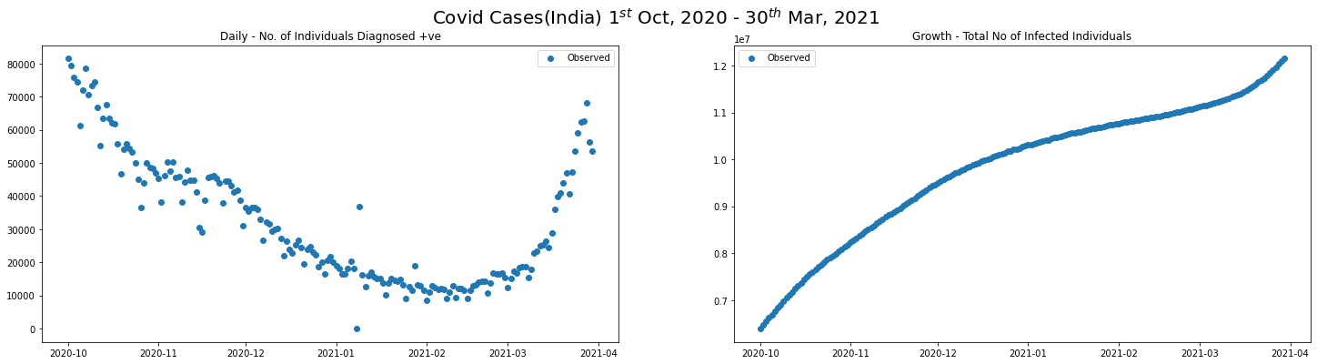
We shall extract the covid new cases and total diagnosed data between October 2020 and March 2021 for understanding Piecewise Linear Regression.
I used univariate spline fit to smooth the data to simplify things
covid_SEP20_MAR21_df = covid_ind_df[(covid_ind_df.date >= "2020-10-01") & (covid_ind_df.date <= "2021-03-30")]
plot_daily_cases(
    covid_SEP20_MAR21_df,
    scatter=True,
    titleA="Daily - No. of Individuals Diagnosed +ve",
    titleB="Growth - Total No of Infected Individuals",
    sup_title="Covid Cases(India) $1^{st}$ Oct, 2020 - $30^{th}$ Mar, 2021"
)

smoothened_data = smooth_spline(covid_SEP20_MAR21_df.new_cases.values, sm_factor=0.1)
covid_SEP20_MAR21_df.loc[:, "new_cases"] = smoothened_data
plot_daily_cases(
    covid_SEP20_MAR21_df,
    scatter=True,
    titleA="Daily - No. of Individuals Diagnosed +ve(Smooth)",
    titleB="Growth - Total No of Infected Individuals",
    sup_title="Covid Cases(India) $1^{st}$ Oct, 2020 - $30^{th}$ Mar, 2021"
)
/Users/shankar/dev/tools/anaconda3/envs/nxt/lib/python3.9/site-packages/pandas/core/indexing.py:1773: SettingWithCopyWarning:
A value is trying to be set on a copy of a slice from a DataFrame.
Try using .loc[row_indexer,col_indexer] = value instead

See the caveats in the documentation: https://pandas.pydata.org/pandas-docs/stable/user_guide/indexing.html#returning-a-view-versus-a-copy
  self._setitem_single_column(ilocs[0], value, pi)
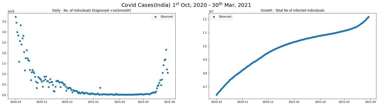
Observe in Pieces
From the graphs we can see, there are 6 different regions where trend shifts during the period between the end of the first wave and the beginning of the second wave.

# !python -m pip install pwlf
Piecewise Linear Regression
We need Piecewise Linear Regression models when the relationship between the dependent variable$(y)$ and the independent variable$(x)$ is continuous and consist of 2 or more linear segments. Then such function is estimated using nonlinear least squares by specifying the number of segments. Let us say the model fit consist of $k$ linear segment(in our example it is 6) then, $$\Large y = \beta_0 + \beta_1 x + \sum_{j=1}^{k-1} \beta_{j+1}(x - \Delta_j)I(x - \Delta_j) \tag{1. Piecewise Linear Regression Model}$$ Where,
- ${\beta_0}$ is the $y$-intercept
- ${\beta_j}$ is the slope of the segment, ${j=1,2,3, \cdots, k}$
- $\Delta_j$ location of the slope changes between segment $j$ and segment $j+1$
- $I(x-\Delta_j) = 1 \ if \ x \geq \Delta_j$ and $0$ otherwise
import pwlf
pwlf_model = pwlf.PiecewiseLinFit(np.arange(len(covid_SEP20_MAR21_df)), covid_SEP20_MAR21_df.new_cases.values)
z = pwlf_model.fit(5)
slopes = pwlf_model.calc_slopes()

# Predictions
predicted_new_cases = pwlf_model.predict(np.arange(len(covid_SEP20_MAR21_df)))
/Users/shankar/dev/tools/anaconda3/envs/nxt/lib/python3.9/site-packages/pwlf/pwlf.py:1086: RuntimeWarning: invalid value encountered in true_divide
  self.slopes = np.divide(
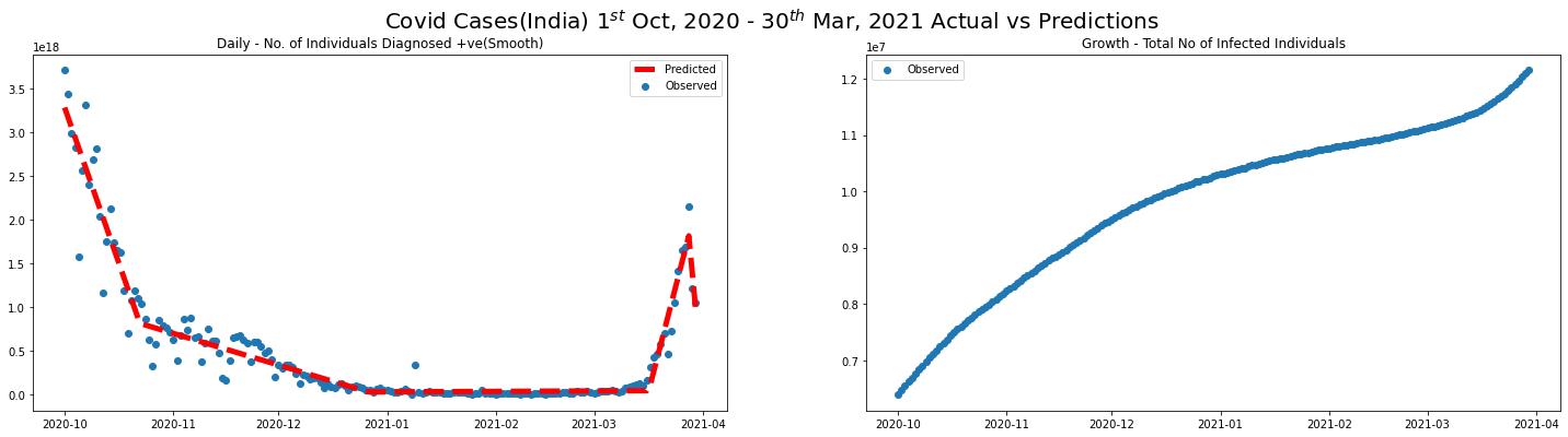
plot_daily_cases(
    covid_SEP20_MAR21_df,
    scatter=True,
    predictions_daily=predicted_new_cases,
    titleA="Daily - No. of Individuals Diagnosed +ve(Smooth)",
    titleB="Growth - Total No of Infected Individuals",
    sup_title="Covid Cases(India) $1^{st}$ Oct, 2020 - $30^{th}$ Mar, 2021 Actual vs Predictions"
)
Exponential and Logarithmic Curve Fitting
We know a simple linear regression model is represented as $y = Ax + B$ and we have studied the Piecewise Linear Regression model in the previous section. An exponential curve fitting model is represented as follows,
$$\Large y = Ae^{Bx} \tag{2. An Exponential Model}$$ $$take \ log \ on \ both \ sides$$ $$log(y) = log(Ae^{Bx}) = log(A) + log(e^{Bx}))$$ $$log(y) = log(A) + Bx$$
Let us do the following,
- Subset the data for a period where there is an exponential growth
- Fit the model using
numpy.polyfitfunction - Apply piecewise linear regression for the
log(y)
Yes, It is a hack but the intent of this post is to understand the idea behind the Piecewise approach and nothing beyond
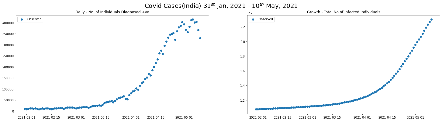
covid_2nd_wave_df = covid_ind_df[(covid_ind_df.date >= "2021-01-31") & (covid_ind_df.date <= "2021-05-10")]
plot_daily_cases(
    covid_2nd_wave_df,
    scatter=True,
    titleA="Daily - No. of Individuals Diagnosed +ve",
    titleB="Growth - Total No of Infected Individuals",
    sup_title="Covid Cases(India) $31^{st}$ Jan, 2021 - $10^{th}$ May, 2021"

)
NUM_PIECES = 10
def logarithmic_fit(data):
    prediction_coeffs = np.polyfit(
        np.arange(len(data)),
        np.log(data.total_cases),
        1,
        w= np.sqrt(data.total_cases)
    )
    B, A = prediction_coeffs

    preds = [np.exp(A) * np.exp(B * x) for x in np.arange(len(data))]

    return preds

def piecewise_logarithmic_fit(data, num_pieces=NUM_PIECES):

    piece_length = len(data) // num_pieces

    predictions = []
    for i in np.arange(num_pieces):
        offset = i * piece_length
        piece_of_data = data[offset:offset + piece_length ]
        preds = logarithmic_fit(piece_of_data)
        predictions.append(preds)

    predictions = np.concatenate(predictions)

    return predictions
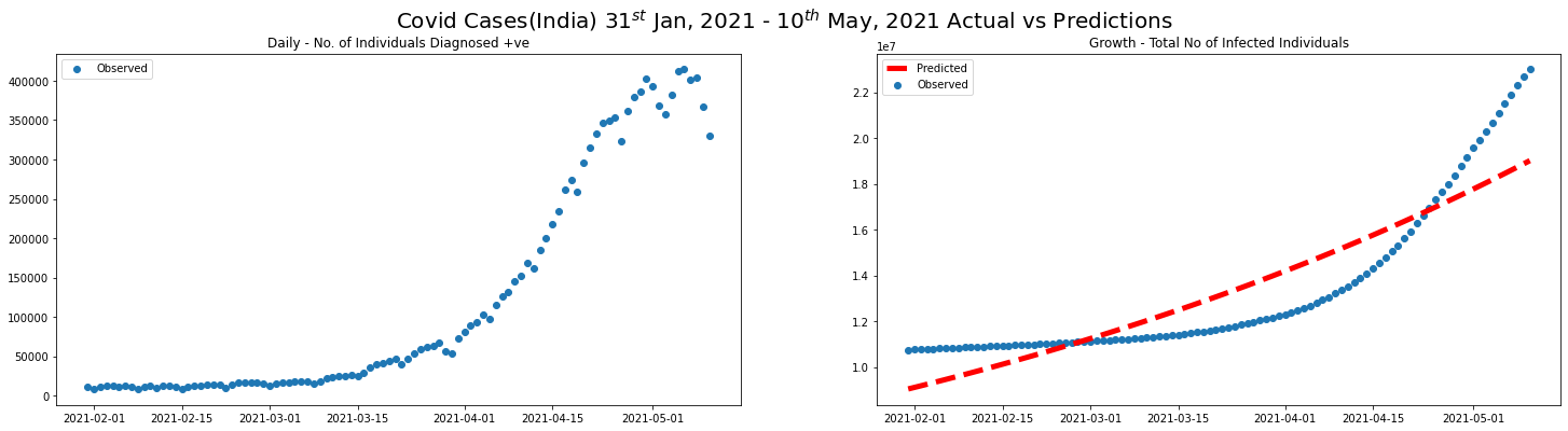
preds = logarithmic_fit(covid_2nd_wave_df)
plot_daily_cases(
covid_2nd_wave_df,
scatter=True,
predictions_total=preds,
titleA="Daily - No. of Individuals Diagnosed +ve",
titleB="Growth - Total No of Infected Individuals",
sup_title="Covid Cases(India) $31^{st}$ Jan, 2021 - $10^{th}$ May, 2021 Actual vs Predictions"
)
pwlf_model = pwlf.PiecewiseLinFit(np.arange(len(covid_2nd_wave_df)), covid_2nd_wave_df.new_cases.values)
z = pwlf_model.fit(5)
slopes = pwlf_model.calc_slopes()
# Predictions
predicted_new_cases = pwlf_model.predict(np.arange(len(covid_2nd_wave_df)))
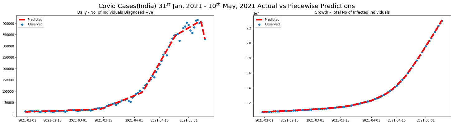
preds = piecewise_logarithmic_fit(covid_2nd_wave_df)
plot_daily_cases(
covid_2nd_wave_df,
scatter=True,
predictions_daily=predicted_new_cases,
predictions_total=preds,
titleA="Daily - No. of Individuals Diagnosed +ve",
titleB="Growth - Total No of Infected Individuals",
sup_title="Covid Cases(India) $31^{st}$ Jan, 2021 - $10^{th}$ May, 2021 Actual vs Piecewise Predictions"
)
/Users/shankar/dev/tools/anaconda3/envs/nxt/lib/python3.9/site-packages/pwlf/pwlf.py:1086: RuntimeWarning: invalid value encountered in true_divide
  self.slopes = np.divide(
Epilogue
In this post, we took one of the most fundamental concepts of machine learning and analyzed using the covid data. Our goal was to learn how the piecewise approach works to get an intuition of polyhedron(cell) in the complex and large-scale DNNs. I took many shortcuts, assumptions, and presumptions to make this post concise and precise at the expense of accuracy/correctness - I request the readers to pardon me for this approach. In my defense, complete learning and understanding a complex concept is a continuous process because we all are in different stages of comprehension. Hoping this post is a useful one that declutters a few critical ideas.
3rd-wave-in-india-covid-debacle-continues-let-us-use-covid-data-to-learn-piecewise-lr-and-exponential-curve-fitting
References
- Piecewise Linear Regression from StatGraphics Centurion, 2020
- How to do exponential and logarithmic curve fitting in Python? I found only polynomial fitting by Kennytm, 2010
- Fit piecewise linear functions to data! from PWLF Library